Navigating Uncertainty: A Critical Analysis of Uncertainty Factors in Ecological Risk Assessment Quotients for Pharmaceutical Development

Abstract

This article provides a comprehensive analysis of uncertainty factors (UFs) within the hazard quotient (HQ) method for ecological risk assessment (ERA), tailored for researchers and drug development professionals. It explores the foundational principles and historical application of UFs, revealing inconsistencies in their implementation and a reliance on often-arbitrary default values[citation:1][citation:8]. The review details contemporary methodological approaches, including probabilistic and data-driven techniques to derive chemical-specific adjustment factors, moving beyond traditional defaults[citation:2][citation:6]. It addresses significant challenges in applying and validating UFs, such as issues with data quality, non-commutability in external quality assessment, and model selection[citation:3][citation:5][citation:7]. Finally, the article compares validation strategies and uncertainty quantification methods, emphasizing the critical need for transparency and scientific rigor. This synthesis aims to enhance the reliability and defensibility of environmental safety assessments for pharmaceuticals.

Understanding the Bedrock: Core Concepts and Historical Evolution of Uncertainty Factors in Risk Quotients

Defining the Hazard Quotient (HQ) and the Role of Uncertainty Factors (UFs)

Technical Support & Troubleshooting Hub

Welcome to the Technical Support Center for Hazard Quotient and Uncertainty Factor applications. This resource is designed for researchers, scientists, and drug development professionals engaged in ecological and human health risk assessment quotient research. The following guides and FAQs address common calculation, interpretation, and methodological challenges.

Core Concepts & Calculation Protocols

The Hazard Quotient (HQ) is a primary screening-level tool used to characterize noncancer risk. It is defined as the ratio of a single substance's potential exposure to a level at which no adverse effects are expected [1] [2].

Fundamental HQ Equation: HQ = Exposure / Reference Value

A HQ less than or equal to 1 indicates that adverse effects are not likely to occur, while a HQ greater than 1 suggests potential risk, though it is not a statistical probability of harm [3] [1].

Key Reference Values: Reference values, such as the Reference Dose (RfD) or Reference Concentration (RfC), are derived from toxicological points of departure (e.g., NOAEL, LOAEL, BMDL) divided by a composite Uncertainty Factor (UF) [3] [2]. RfD = NOAEL / (UFs) [4]

The product of Uncertainty Factors (UFs) is applied to account for various extrapolations and data gaps, including interspecies differences (animal-to-human) and intraspecies variability (within humans) [4] [5].

Comparison of Common Quotient Methods: The table below summarizes the primary quotient methods used in human health and ecological risk assessments.

Assessment Aspect	Hazard Quotient (HQ) for Human Health [4] [3] [1]	Risk Quotient (RQ) for Ecological Risk [1]
Primary Use	Assessing health risks of air toxics, contaminants, and industrial chemicals.	Assessing ecological risks of pesticides and environmental contaminants.
Core Equation	HQ = Exposure Concentration / Reference Concentration (RfC) or Reference Dose (RfD).	RQ = Estimated Environmental Concentration (EEC) / Toxicity Endpoint (e.g., LC50, NOEC).
Point of Departure	Derived from a human-equivalent reference value (RfD/RfC) which already incorporates UFs.	Uses a raw ecotoxicity endpoint from studies on algae, invertebrates, or fish.
Risk Threshold	HQ ≤ 1: Negligible hazard likely. HQ > 1: Potential for adverse effects increases.	Compared to a Level of Concern (LOC). E.g., for chronic risk, RQ must be < LOC of 1.0 [1].
Role of UFs	UFs are embedded within the RfD/RfC used in the denominator.	UFs or Assessment Factors may be applied separately to the toxicity endpoint or are considered within the LOC.

Detailed Methodological Guides

1. Protocol for Probabilistic Derivation of Chemical-Specific Uncertainty Factors

This data-driven protocol aims to replace default UFs with chemical-specific assessment factors where sufficient data exist [5].

• Objective: To derive empirical distributions for specific UF components (e.g., interspecies, intraspecies, LOAEL-to-NOAEL) using existing toxicity data for a chemical category.
• Materials: A curated database of toxicity values (e.g., NOAELs, LOAELs, LD₅₀s) for the chemical(s) of interest, ideally from standardized studies.
• Procedure: a. Data Compilation: Gather all relevant pairwise toxicity data (e.g., acute LD₅₀ to chronic NOAEL ratios for Acute-to-Chronic Ratios; subchronic to chronic NOAELs for duration extrapolation) [5]. b. Ratio Calculation: For each pair of data points, calculate the required ratio (e.g., LOAEL:NOAEL). c. Distribution Fitting: Use statistical software to fit a distribution (e.g., log-normal) to the calculated ratios. d. Percentile Selection: Identify a protective percentile (e.g., 95th or 99th) of the distribution. The value at this percentile may be proposed as a data-derived UF [5] [6]. e. Uncertainty Analysis: Perform Monte Carlo simulations to characterize uncertainty in the derived UF and calculate confidence intervals [5].
• Troubleshooting: If the dataset is too small for reliable distribution fitting, consider read-across from a similar chemical category or revert to a relevant default UF [5].

2. Protocol for Calculating Aggregate Risk with Hazard Index (HI) for Mixtures

This protocol assesses cumulative risk from exposure to multiple chemicals affecting the same target organ [1] [2].

• Objective: To calculate a Hazard Index (HI) to evaluate the combined risk from a mixture of chemicals.
• Principle: The HI is the sum of the individual HQs for chemicals that share a common mechanism of toxicity or affect the same critical organ system [7] [2]. HI = Σ (HQ₁ + HQ₂ + ... + HQₙ)
• Procedure: a. Grouping: Identify all chemicals in the mixture for which exposure data exists. Group them based on a common critical adverse effect or mode of action [7]. b. Individual HQ Calculation: Calculate the HQ for each chemical as described in the Core Concepts. c. Summation: Sum the HQs for all chemicals within the defined group. d. Interpretation: An HI ≤ 1 suggests negligible risk from the mixture. An HI > 1 indicates potential for additive effects and requires further, more refined assessment [2].
• Critical Note: A significant limitation arises when adding HQs based on Reference Doses (RfDs) derived from different critical adverse effects. This can lead to misleading risk estimates [7]. The Adversity Specific Hazard Index (HIA) approach is recommended, where summation is only performed for chemicals whose RfDs are based on the identical critical effect [7].

Troubleshooting: Visualization of Workflows and Relationships

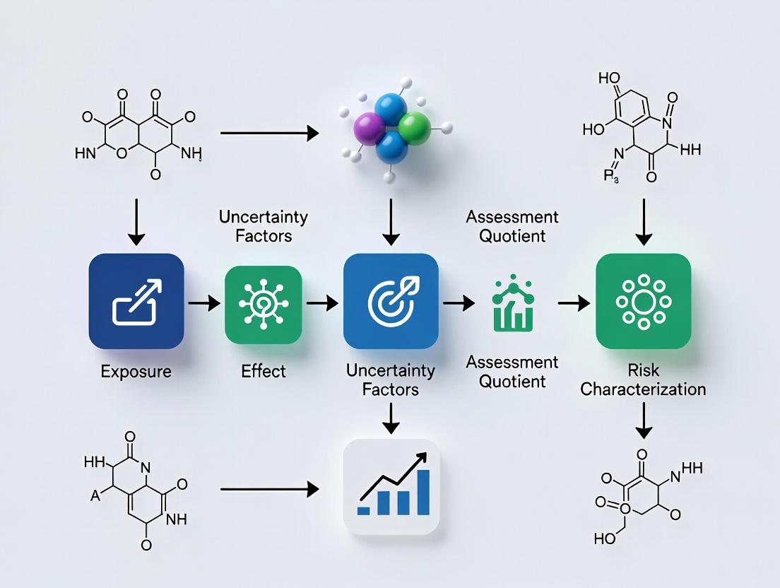
Diagram 1: Workflow for HQ Calculation & Risk Characterization

Diagram 2: Role & Composition of Uncertainty Factors (UFs)

The Scientist's Toolkit: Research Reagent Solutions

Item / Solution	Function in Hazard & Risk Assessment Research
Toxicological Points of Departure (NOAEL, LOAEL, BMDL)	Serve as the experimental benchmark from animal or in vitro studies from which safe human limits are extrapolated [5] [3].
Chemical-Specific Toxicity Databases	Curated databases (e.g., for LD₅₀, NOAEL values) are essential raw materials for probabilistic UF derivation and Threshold of Toxicological Concern (TTC) approaches [5].
Probabilistic Distribution Software	Tools for Monte Carlo simulation and fitting log-normal distributions are required to empirically derive UFs from toxicity data ratios and quantify uncertainty [5].
Exposure Assessment Models	Models to generate Estimated Environmental Concentrations (EECs) or Estimated Human Exposures (EHEs) are needed for the numerator in HQ/RQ calculations [1].
Consensus Reference Values (RfD, RfC, ADI)	These are the finalized "reagents" for risk characterization, integrating the toxicological POD with standard or chemical-specific UFs [3] [2].

Frequently Asked Questions (FAQs)

Q1: My calculated HQ is 2.5. Does this mean there is a 250% chance of adverse effects? A: No. The HQ is not a probabilistic measure of risk [3] [1]. A HQ > 1 indicates that the exposure level exceeds the reference level (RfD/RfC). It is a signal that potential for risk exists and that further investigation or more refined assessment is warranted. It does not quantify the likelihood or severity of the effect.

Q2: When should I use a chemical-specific UF instead of the default 10x factors? A: Use chemical-specific or data-derived UFs when you have robust, quantitative data to inform a specific extrapolation [5] [6]. For example:

• Toxicokinetic Data: If you have in vivo or in vitro data comparing metabolism or clearance between test species and humans.
• Toxicodynamic Data: If you understand the mode of action and have comparative data on target receptor sensitivity.
• Chemical Category Data: If you have sufficient toxicity data across a group of similar chemicals to perform a probabilistic analysis as described in the protocols above [5]. If such data are lacking, the default factors (e.g., 10 for interspecies, 10 for intraspecies) should be applied as they are considered protective.

Q3: How do I handle HQ calculations for a chemical mixture from a single source (e.g., pesticides in one food item)? A: The standard Hazard Index (HI) approach may underestimate risk if it doesn't account for aggregate exposure from all sources [7]. For single-source assessments, consider the Source-Related Hazard Quotient (HQs) approach [7]:

• Calculate HQs normally (exposure from the source / ADI).
• Determine a Correction Factor (CF) representing the maximum permitted contribution of that source to total dietary exposure.
• Compare the HQs to the CF, not to 1. A risk is indicated if HQs > CF [7]. This method provides a more realistic risk characterization when only single-source data is available.

Q4: What is the most common error in interpreting the Hazard Index (HI) for mixtures? A: The most common error is summing HQs for chemicals whose Reference Doses are based on different critical adverse effects [7]. For example, adding an HQ for a chemical with an RfD based on liver toxicity to an HQ for a chemical with an RfD based on developmental toxicity is not scientifically supportable. Always verify the "critical effect" for each chemical's RfD and sum HQs only for chemicals that affect the same target organ or system, ideally via a similar mode of action. The Adversity Specific Hazard Index (HIA) methodology is designed to correct this error [7].

This technical support center provides resources for researchers conducting Ecological Risk Assessment (ERA) quotient research, a field grounded in deterministic methods but evolving towards structured uncertainty analysis. For decades, risk quotients (RQs)—calculated by dividing a point estimate of exposure by a point estimate of effect—have served as a primary screening-level tool [8] [9]. To account for unknowns, default uncertainty factors (UFs), often 10-fold values, have been applied [5]. This practice originated in the 1950s with food and pesticide safety assessments [10].

However, this "one-size-fits-all" approach contains significant, unquantified uncertainty and may not reflect specific chemical or ecological contexts [9]. Modern research emphasizes moving beyond default factors to structured uncertainty analysis. This involves probabilistic methods, chemical-specific adjustment factors (CSAFs), and frameworks like the Scenario–Model–Parameter (SMP) approach, which systematically accounts for multiple uncertainty sources [5] [11]. This evolution forms the thesis of modern ERA: transitioning from generic safety margins to transparent, quantitative, and hypothesis-driven uncertainty characterization.

Core Methodologies & Technical Reference

Standard Risk Quotient (RQ) Calculations

The deterministic RQ method is the baseline for screening-level assessments. The core formula is RQ = Exposure / Toxicity [8]. The specific parameters vary by assessed organism and exposure scenario.

Table: Standard Risk Quotient Formulas by Organism Type [8]

Organism Group	Assessment Type	Exposure Estimate (EEC)	Toxicity Endpoint	Formula
Terrestrial Animals (Birds/Mammals)	Acute Dietary	Estimated Environmental Concentration (EEC) in mg/kg-diet	Lowest LD50 (oral)	Acute RQ = EEC / LD50
	Chronic Dietary	EEC in mg/kg-diet	Lowest NOAEL (mg/kg-diet)	Chronic RQ = EEC / NOAEL
Aquatic Animals	Acute	Peak Water Concentration	Most sensitive LC50 or EC50	Acute RQ = Peak Concentration / LC50
	Chronic (Fish)	56- or 60-day Avg. Water Concentration	Early Life-Stage NOAEC	Chronic RQ = Avg. Concentration / NOAEC
Terrestrial Plants	Acute (Non-listed)	EEC from Runoff + Spray Drift	EC25 (Seedling Emergence)	RQ = EEC / EC25
Aquatic Plants	Acute (Non-listed)	EEC in water	Lowest EC50 (Algae/Vascular)	RQ = EEC / EC50

Uncertainty Factor (UF) Application Protocol

When a Risk Quotient (RQ) indicates potential risk, Uncertainty Factors (UFs) are applied to derive a "safe" concentration or dose. The general equation is: Adjusted Reference Value = Point of Departure (NOAEL, BMDL, etc.) / (UF₁ × UF₂ × ... × UFₙ) [10].

Table: Common Uncertainty Factors and Their Rationale [5] [10]

Uncertainty Factor (UF)	Area of Uncertainty Addressed	Typical Default Value	Purpose & Notes
UFA	Interspecies (Animal to Human)	10	Accounts for differences in toxicokinetics/toxicodynamics between test species and humans. Can be subdivided (e.g., 4.0 for TK, 2.5 for TD) [5].
UFH	Intraspecies (Human Variability)	10	Protects sensitive human subpopulations. May be partitioned similarly to UFA [10].
UFS	Subchronic to Chronic Extrapolation	1-10	Applied when the Point of Departure is from a less-than-lifetime study.
UFL	LOAEL to NOAEL Extrapolation	1-10	Applied when the critical study identifies a LOAEL instead of a NOAEL.
UFD	Database Incompleteness	1-10	Reflects deficiencies in the overall toxicity database (e.g., missing studies, endpoints).
MF	Modifying Factor	≤1 to 10	A professional judgment factor accounting for additional scientific uncertainties not covered by standard UFs [10].

Scenario-Model-Parameter (SMP) Uncertainty Analysis Protocol

The SMP framework is a advanced, multi-step procedure for cumulative risk assessment that moves beyond parameter-only uncertainty [11].

Experimental Protocol: SMP Uncertainty Analysis [11]

• Identify toxic effects and endpoints for all chemicals sharing a common mechanism of toxicity.
• Identify exposure scenarios of concern (e.g., multiple routes, populations, timeframes).
• Develop dose models for each exposure route (inhalation, ingestion, dermal).
• Estimate exposure, dose, and risk using the selected models and scenarios.
• Perform uncertainty analyses:
  • Parameter Uncertainty: Use Monte Carlo simulation to vary input parameters (e.g., body weight, ingestion rate).
  • Model Uncertainty: Run steps 1-4 using two or more equally plausible mathematical models.
  • Scenario Uncertainty: Run steps 1-4 under two or more equally plausible exposure scenarios.
• Characterize risk by comparing the probability distributions of risk estimates generated from parameter-only uncertainty versus the combined SMP uncertainty. This identifies if ignoring model/scenario sources meaningfully underestimates total uncertainty.

The Scientist's Toolkit: Research Reagent Solutions

Table: Essential Materials for ERA & Uncertainty Research

Item / Reagent	Primary Function in ERA Research	Application Notes
Standard Toxicity Test Organisms (e.g., Fathead minnow, Daphnia magna, Rat, Quail)	Generate foundational LC50, EC50, NOAEL, and LOAEL data for RQ calculation [8].	Required for regulatory submissions. Choice of species is critical for extrapolation relevance.
Chemical-Specific Toxicokinetic/Toxicodynamic (TK/TD) Data	Enables replacement of default UFs with Chemical-Specific Adjustment Factors (CSAFs) [5] [10].	Obtained from in vitro assays, PBPK models, or biomarker studies. Key for modern, data-driven assessments.
Probabilistic Exposure Modeling Software (e.g., T-REX, TerrPlant [8])	Generates exposure concentration distributions (EECs) for probabilistic risk assessment, moving beyond single point estimates.	Models are scenario-driven. Understanding model algorithms and input requirements is essential for uncertainty analysis.
Statistical Software for Dose-Response Modeling (e.g., for Benchmark Dose, BMD, analysis)	Determines a Point of Departure (POD) with associated confidence intervals, superior to using a NOAEL from a single test dose [10].	BMD modeling uses all dose-response data, providing a more robust and quantitative POD for UF application.
Monte Carlo Simulation Software	Propagates variability and uncertainty in exposure and toxicity parameters to generate a probability distribution of risk [11].	Core tool for implementing parameter uncertainty analysis in the SMP framework and probabilistic ecological risk assessment.

Troubleshooting Guides & FAQs

FAQ 1: When should I use a default Uncertainty Factor (UF) versus developing a Chemical-Specific Adjustment Factor (CSAF)?

• Issue: Concern that a default 10-fold UF may be overly conservative or, conversely, insufficiently protective for a specific chemical.
• Solution: Use default UFs during initial screening-level assessments or when chemical-specific data are utterly lacking [10]. Develop and apply a CSAF when data exist to characterize interspecies differences (e.g., in vitro metabolism studies) or human variability (e.g., genetic polymorphism data) [5]. The trend in regulatory science is to replace defaults with CSAFs whenever possible to increase transparency and scientific rigor [10].

FAQ 2: My Risk Quotient (RQ) is marginally above the Level of Concern (LOC). What are the most defensible refinements?

• Issue: A screening-level RQ > 1.0 triggers regulatory concern, but may be based on overly conservative assumptions.
• Solution: Follow a tiered refinement strategy:
  • Refine Exposure: Replace generic estimates with chemical-specific fate data or monitored environmental concentrations. Use probabilistic modeling to represent exposure distributions [9].
  • Refine Effects: Consider using a Benchmark Dose (BMD) instead of a NOAEL, or evaluate toxicity for a more relevant, locally present species [10].
  • Refine the Assessment Framework: For chronic or population-level risks, consider moving from the RQ to a mechanistic population model (e.g., following Pop-GUIDE) that integrates life-history traits and ecological relevance [9].

FAQ 3: How do I quantitatively incorporate model and scenario uncertainty, not just parameter uncertainty?

• Issue: Traditional Monte Carlo analysis only addresses parameter uncertainty, potentially underestimating total uncertainty.
• Solution: Implement the Scenario-Model-Parameter (SMP) Uncertainty Analysis [11].
  • Protocol: See Section 2.3. Systematically run your assessment using alternate, equally plausible models (e.g., different exposure algorithms) and scenarios (e.g., different land-use or behavioral assumptions).
  • Outcome: Compare the risk distribution from the parameter-only analysis to the combined SMP analysis. If the SMP distribution is significantly broader, model/scenario uncertainty is critical and must be reported to risk managers.

FAQ 4: What are the major pitfalls in interpreting a probabilistic risk assessment?

• Issue: Misinterpreting the output of a Monte Carlo simulation or probabilistic population model.
• Solution:
  • Do not treat the mean or median risk estimate as a deterministic "answer." The entire distribution (e.g., the 5th to 95th percentile range) characterizes uncertainty.
  • Clearly communicate that the assessment is based on a set of defined scenarios and models. Different assumptions will yield different results.
  • Ensure transparency by fully documenting all input distributions, model choices, and scenario definitions. The value lies in the comparative analysis of assumptions, not a single "true" risk number [11] [9].

FAQ 5: The historical default of a 10-fold safety factor seems arbitrary. What is its scientific basis and is it still valid?

• Issue: The origin and justification for the 10x UF are unclear, leading to questions about its applicability.
• Solution: Recognize its historical and policy context. The 100-fold factor (10 each for inter- and intra-species) was first proposed in 1954 by Lehman and Fitzhugh as a pragmatic "margin of safety" for food additives [10]. Subsequent analyses, like Renwick's work in the 1990s, provided a partial scientific basis by partitioning it into sub-factors for toxicokinetics (4.0) and toxicodynamics (2.5) [5]. Its validity today is conditional: It remains a necessary, health-protective default in the absence of data. However, it is not a substitute for chemical-specific investigation. Modern best practice is to use the default UF as a starting point to be reduced or replaced as data permit [5] [10].

Technical Support & Troubleshooting Hub

FAQ & Troubleshooting Guide: Applying Uncertainty Factors (UFs) in Ecological Risk Assessment Quotients

Q1: I am extrapolating from a mammalian lab species (e.g., rat) to a non-target wildlife species (e.g., bird) in my risk quotient calculation. Which Interspecies UF should I apply, and what are the common pitfalls? A: The standard default Interspecies UF is 10. This is typically bifurcated into subfactors for toxicokinetic (TK, 4.0) and toxicodynamic (TD, 2.5) differences (10 ≈ 4.0 * 2.5). A common error is applying the full UF 10 when chemical-specific adjustment factors (CSAFs) are available. Troubleshooting: If you have in vitro metabolism data (Vmax, Km) or protein-binding data for both species, you can derive a chemical-specific TK factor to replace the default of 4.0. Failure to use available data may overestimate uncertainty. Consult the IPCS framework for CSAFs.

Q2: My chronic toxicity study was only 28 days long, but I need to assess lifetime exposure for a long-lived species. How do I correctly apply the Duration Extrapolation UF? A: The default Duration UF for subchronic-to-chronic extrapolation is 10. The primary issue is misapplication when the available study is actually of chronic duration. Troubleshooting: First, confirm the study duration relative to the species' lifespan. A 28-day study in rodents is subchronic. For fish early life stage tests, a UF may still be needed to account for full life-cycle effects. Ensure your exposure scenario justifies chronic extrapolation. If multiple subchronic studies show consistent effects, consider a reduced UF (e.g., 3-5) with justification.

Q3: I only have a LOAEL from my key study, not a NOAEL. What is the correct methodology for applying the LOAEL-to-NOAEL UF? A: The standard default UF is 10. The core problem is arbitrary application without assessing the "severity" of the LOAEL. Troubleshooting: Analyze the dose-response gradient. If the LOAEL is associated with only minimal, adaptive effects (e.g., slight, transient enzyme induction), a lower factor (e.g., 3) may be scientifically defensible. Alternatively, you can use benchmark dose (BMD) modeling on the raw data to derive a point of departure, which may circumvent the need for this UF entirely. Always document the severity of the effect at the LOAEL.

Q4: My toxicity database for the chemical has gaps (e.g., missing reproductive toxicity data for aquatic invertebrates). How do I quantify and apply the Database Insufficiency UF? A: There is no single default value; it is based on a weight-of-evidence assessment. The error is applying an arbitrary factor (e.g., 10) without structured analysis. Troubleshooting: Use a Modified Scoring System. Evaluate missing taxa (e.g., algae, daphnia, fish) and missing endpoints (acute, chronic, reproduction). Assign scores for each gap (see Table 1). The composite score guides the UF magnitude. A partial UF (e.g., 2-5) is often used for a specific, critical gap rather than a blanket factor.

Table 1: Database Insufficiency UF Scoring Guidance

Database Gap	Severity Score	Recommended UF Range	Notes
Missing a major trophic level (e.g., no aquatic plant data)	High (3)	3 - 10	Critical for herbicides; UF at higher end.
Missing chronic data for a key representative species	High (3)	3 - 10	Required for long-term risk assessment.
Only acute data for all taxa	Moderate (2)	2 - 5	Limits capacity for chronic RQ derivation.
Missing a specific endpoint (e.g., reproduction) in an otherwise robust chronic study	Low (1)	1 - 3	May apply a small additional factor.
Complete data for all standard laboratory taxa	None (0)	1	No additional UF warranted.

Experimental Protocols for Key Studies

Protocol 1: Deriving Chemical-Specific Adjustment Factors (CSAFs) for Interspecies Extrapolation Objective: To replace default TK/TD UFs with data-derived values. Methodology:

• Toxicokinetics (TK):
  • Conduct in vitro metabolism studies using hepatic S9 or microsomal fractions from the laboratory species (rat) and the target wildlife species (e.g., bird liver).
  • Determine kinetic parameters (Km, Vmax) for the chemical's major metabolic pathway.
  • Calculate the Relative Metabolic Rate = (Vmax/Km)~human~ / (Vmax/Km)~rat~.
  • The inverse of this ratio can inform the TK component of the interspecies UF.
• Toxicodynamics (TD):
  • Identify the molecular target (e.g., enzyme, receptor).
  • Compare in vitro sensitivity (e.g., IC50, Ki) of the target protein between species using purified proteins or cell lines.
  • The ratio of sensitivities informs the TD component. Analysis: The composite CSAF = TK factor × TD factor. This replaces the default 10.

Protocol 2: Benchmark Dose (BMD) Modeling to Replace LOAEL-to-NOAEL Extrapolation Objective: To derive a POD without relying on the LOAEL/NOAEL dichotomy. Methodology:

• Obtain the raw dose-response data from the toxicity study.
• Select a suite of mathematical models (e.g., log-logistic, quantal-linear, Weibull) in software (e.g., EPA BMDS, PROAST).
• Fit all models to the data, specifying a critical benchmark response (BMR), typically a 10% extra risk for quantal data or a 1 standard deviation change for continuous data.
• Calculate the BMD confidence interval (BMDL, BMDU).
• Select the BMDL (lower confidence limit) as the POD. Analysis: The BMDL is used directly in the risk quotient (RQ = PEC / BMDL). This approach is scientifically rigorous and often eliminates the need for the LOAEL-to-NOAEL UF.

Visualizations

Title: Uncertainty Factor Application Decision Workflow

Title: Interspecies UF Covers TK and TD Variability

The Scientist's Toolkit: Research Reagent Solutions

Reagent / Material	Function in UF-Related Research
Hepatic S9 Fractions or Microsomes (from human, rat, bird, fish)	Used in in vitro metabolism studies to derive chemical-specific toxicokinetic data for Interspecies CSAF calculation.
Species-Specific Target Proteins (e.g., recombinant enzymes, receptors)	For comparing toxicodynamic sensitivity between species via IC50/Ki assays, informing the TD component of the Interspecies UF.
Benchmark Dose (BMD) Software (e.g., EPA BMDS, R package drc)	Enables dose-response modeling to derive a BMDL, eliminating the need for the LOAEL-to-NOAEL UF and providing a more robust POD.
Standardized Test Organism Cultures (e.g., Daphnia magna, Pseudokirchneriella subcapitata, fathead minnow embryos)	Essential for filling database gaps. Chronic life-cycle tests with these species can reduce or eliminate the Database Insufficiency UF.
High-Throughput Screening (HTS) Assays (e.g., ToxCast/Tox21 assays)	Provides preliminary data on multiple biological pathways across taxa, helping to identify critical data gaps and prioritize testing for Database UF assessment.
Physiologically Based Toxicokinetic (PBTK) Modeling Software (e.g., GastroPlus, Simcyp)	Allows extrapolation of internal dose across species and life stages using physiological parameters, refining the Interspecies and Duration UF application.

Technical Support Center: Troubleshooting Default Values in Ecological Risk Assessment (ERA)

This technical support center assists researchers, scientists, and drug development professionals in navigating the establishment, application, and inherent limitations of default values within Ecological Risk Assessment (ERA) quotient methods. Operating within the broader thesis context of uncertainty factors in ecological risk assessment research, this guide provides targeted troubleshooting for common experimental and interpretive challenges [9].

Frequently Asked Questions (FAQs)

FAQ 1: What is a default value in ERA, and why is it used? A default value is a standardized, conservative parameter used in screening-level ecological risk assessments when chemical- or species-specific data are lacking [9]. The most common default is the Risk Quotient (RQ), calculated as the ratio of an Estimated Environmental Concentration (EEC) to a Toxicity Endpoint (e.g., LC50, NOAEC) [8]. Defaults provide a consistent, initial screening tool to prioritize chemicals and scenarios requiring more refined, resource-intensive assessment [9].

FAQ 2: My Risk Quotient (RQ) exceeds the Level of Concern (LOC). What are my next steps? An RQ > LOC indicates a potential risk at the screening level. Your next steps involve tiered refinement to reduce uncertainty [9]:

• Refine Exposure Estimates: Replace generic model defaults with site-specific data (e.g., local application rates, soil types, water bodies).
• Refine Effects Data: If available, use toxicity data for more relevant, sensitive local species or life stages instead of standard test species.
• Consider Probabilistic Approaches: Move beyond single-point RQs to use full exposure and effects distributions for a probabilistic risk estimate [9].
• Consult Higher-Tier Models: Explore the use of mechanistic population models (e.g., following Pop-GUIDE) to understand ecological relevance [9].

FAQ 3: How are the specific toxicity endpoint defaults (e.g., LC50, NOAEC) selected for different species? Regulatory guidelines prescribe standard test species and endpoints for consistency. The selected default is typically the most sensitive endpoint (lowest value) from a suite of required toxicity tests for a given assessment type [8]. See Table 1 for standard endpoints.

FAQ 4: What are the major sources of uncertainty when using default RQ methods? Key uncertainties are inherent in both components of the RQ [9]:

• Exposure (EEC): Temporal/spatial averaging obscures peak exposures; point estimates ignore variable exposure profiles [9].
• Effects (Toxicity): Laboratory-to-field extrapolation; single-species tests to community/population impacts; acute-to-chronic extrapolation [9].
• The Quotient Itself: A scalar RQ cannot quantify probability, magnitude of effect, or recoverability. It conflates different exposure/effect distribution shapes into a single number [9].

FAQ 5: How can I effectively communicate the limitations of default-value assessments in my research reports? Adhere to the TCCR principles (Transparent, Clear, Consistent, Reasonable) for risk characterization [8]. Explicitly:

• State that the assessment is a screening-level tool.
• List all default values and assumptions used.
• Qualify conclusions by describing the conservative nature of defaults.
• Recommend specific avenues for refinement (e.g., "A probabilistic assessment is recommended to characterize the likelihood of effects given the variable exposure pattern") [9].

Troubleshooting Guide: Common Experimental & Analytical Issues

Problem 1: Inconsistent or Unclear Risk Characterization Conclusions

• Symptoms: Difficulty determining "pass/fail"; contradictory interpretations of the same RQ value; feedback indicates results are not useful for decision-making [8].
• Root Cause: Lack of adherence to a structured risk characterization framework.
• Solution:
  • Ensure your risk characterization integrates exposure and effects analyses clearly [8].
  • Explicitly describe all uncertainties, assumptions, and the strengths/limitations of the data [8].
  • Synthesize a clear conclusion about risk using the TCCR principles [8].
  • Use a standardized report structure (Title, Abstract, Introduction, Methods, Results, Discussion, References) to ensure completeness [12] [13].

Problem 2: The Default Toxicity Endpoint Seems Ecologically Irrelevant for My Assessment Scenario

• Symptoms: The standard lab test species is phylogenetically or functionally distant from the species of concern; the endpoint (e.g., mortality) doesn't align with the assessment goal (e.g., population sustainability).
• Root Cause: Defaults are standardized for broad regulatory application, not specific ecological scenarios [9].
• Solution:
  • Document the Limitation: Clearly state this uncertainty in your assessment [8].
  • Propose a Refined Endpoint: If data exists, justify and use a more relevant endpoint (e.g., a sub-lethal reproduction NOAEC for a population-level assessment) [8].
  • Advocate for Modeling: For higher-tier assessment, propose using a mechanistic population model that can translate individual-level effects to population-relevant metrics [9].

Problem 3: My Calculated RQ is Borderline Relative to the LOC, Making Risk Management Decisions Difficult

• Symptoms: The RQ is slightly above or below the LOC; small changes in input assumptions flip the conclusion.
• Root Cause: Deterministic point estimates do not account for natural variability or measurement uncertainty [9].
• Solution:
  • Conduct Sensitivity Analysis: Systematically vary key input parameters (e.g., application rate, toxicity value) within plausible ranges to see how the RQ changes.
  • Perform Probabilistic Analysis: Use available data to model the EEC and/or toxicity endpoint as distributions (e.g., using @Risk or Crystal Ball software). Calculate the probability that exposure exceeds toxicity.
  • Present a Risk Profile: Instead of a single "pass/fail," present a range of plausible outcomes to support more nuanced decision-making [9].

Experimental Protocols & Methodologies

Protocol 1: Standardized Calculation of Acute and Chronic Risk Quotients (RQs) This protocol outlines the deterministic quotient method as per EPA guidelines [8].

• 1. Objective: To derive a screening-level estimate of risk by comparing a point estimate of exposure to a point estimate of toxicity.
• 2. Materials: See "The Scientist's Toolkit" table.
• 3. Procedure:
  • Step 1 - Exposure Characterization (EEC): Using a fate & transport model (e.g., T-REX for terrestrial, PRZM/EXAMS for aquatic), calculate the relevant EEC. For acute RQs, this is typically a peak concentration (e.g., peak water concentration). For chronic RQs, this is a time-weighted average (e.g., 21-day average for invertebrates, 60-day for fish) [8].
  • Step 2 - Effects Characterization: Obtain the appropriate toxicity endpoint from guideline studies. For acute RQs, this is typically the LC50 or EC50 (for the most sensitive standard test species). For chronic RQs, this is the No Observable Adverse Effect Concentration (NOAEC) [8].
  • Step 3 - Risk Quotient Calculation: Apply the formula: RQ = EEC / Toxicity Endpoint.
  • Step 4 - Risk Estimation: Compare the calculated RQ to the pre-defined Levels of Concern (LOCs). LOCs vary by regulatory agency and species (e.g., USEPA often uses LOC = 0.5 for acute risk to endangered species, 0.1 for chronic risk).
• 4. Reporting: Report the RQ, the LOC, and a clear statement of potential risk. All input values, models, and assumptions must be documented [8] [12].

Protocol 2: Refinement Using a Probabilistic Risk Assessment (PRA) Approach This advanced protocol addresses limitations of deterministic RQs by incorporating variability [9].

• 1. Objective: To estimate the probability and magnitude of adverse ecological effects by integrating distributions of exposure and toxicity.
• 2. Materials: Statistical software (R, Python), Monte Carlo simulation add-ins (@Risk), datasets of exposure concentrations and/or toxicity values.
• 3. Procedure:
  • Step 1 - Develop Distributions: Fit appropriate statistical distributions to exposure data (e.g., modeled or monitored concentrations over time/space) and/or species sensitivity distributions (SSDs) to toxicity data.
  • Step 2 - Monte Carlo Simulation: Run a simulation (e.g., 10,000 iterations). For each iteration, randomly select a value from the exposure distribution and a value from the effects distribution. Calculate a "probabilistic RQ" for that iteration.
  • Step 3 - Analyze Output: The result is a distribution of RQs. Analyze the proportion of iterations where RQ > 1 (or another threshold). This proportion represents the probability of exceeding the effects threshold.
  • Step 4 - Create a Risk Curve: Plot the cumulative probability of effects against the exposure concentration or RQ magnitude.
• 4. Reporting: Report the probability of adverse effects (e.g., "There is a 12% probability that the chronic exposure concentration exceeds the NOAEC for the most sensitive 10% of species"). Include the developed distributions and simulation parameters [9].

Data Presentation: Standard Default Values & Endpoints

Table 1: Standard Toxicity Endpoints Used as Defaults in Screening-Level Risk Quotient Calculations [8]

Assessment Type	Receptor Group	Standard Toxicity Endpoint (Default)
Acute Assessment	Terrestrial Birds & Mammals	Lowest available LD₅₀ (oral) or LC₅₀ (dietary)
Chronic Assessment	Terrestrial Birds & Mammals	Lowest available NOAEC from reproduction test
Acute Assessment	Aquatic Fish & Invertebrates	Lowest available LC₅₀ or EC₅₀ (from acute tests)
Chronic Assessment	Aquatic Invertebrates	Lowest available NOAEC from early life-stage test
Chronic Assessment	Aquatic Fish	Lowest available NOAEC from full life-cycle test
Plant Assessment	Terrestrial & Aquatic Plants	EC₂₅ (for non-listed species) or NOAEC/EC₀₅ (for listed species)

Table 2: Key Uncertainties and Limitations Associated with Default Risk Quotient Methodology [9]

Component	Source of Uncertainty	Consequence for Risk Estimation
Exposure (EEC)	Use of a single high-percentile point estimate (e.g., 90th percentile).	Obscures exposure frequency, duration, and timing relative to species life cycles. May be under- or over-conservative.
Exposure (EEC)	Lack of spatial explicitness.	Cannot identify risk in critical habitats if they don't coincide with the highest average exposure.
Effects (Toxicity)	Use of limited surrogate species.	May not protect all real-world species. Laboratory conditions do not reflect field stressors.
Effects (Toxicity)	Use of individual-level endpoints (mortality, growth).	Difficult to extrapolate to population-level consequences (abundance, extinction risk).
Risk Quotient (RQ)	Scalar, deterministic calculation.	Provides no information on the probability, severity, or reversibility of effects. Two scenarios with the same RQ can have vastly different risks.

Visualizations: Workflows and Relationships

Diagram 1: Tiered Ecological Risk Assessment Workflow with Default Path

Diagram 2: The Science-Policy Interface in Ecological Decision-Making

The Scientist's Toolkit: Research Reagent Solutions

Table 3: Essential Materials and Reagents for Ecological Risk Assessment Research

Item	Function in ERA Research	Key Considerations
Standard Test Organisms(e.g., Fathead minnow, Rainbow trout, Water flea (Daphnia), Earthworm, Zebrafish)	Surrogate species for generating regulatory-accepted toxicity endpoints (LC50, NOAEC) [8].	Maintain cultures under guideline conditions (OECD, EPA). Use consistent age/size classes for test reproducibility.
Formulated Chemical Test Substance	The agent of concern for which toxicity is being characterized.	Use highest purity available. Characterize stability and solubility in test media. Prepare fresh stock solutions as needed.
Reconstituted Water / Standard Soil	Provides a consistent, defined medium for aquatic or terrestrial toxicity tests.	Follow standard recipes (e.g., EPA reconstituted water). Monitor and document key parameters (pH, hardness, temperature, organic matter).
Analytical Grade Solvents & Reagents	For chemical extraction, cleanup, and analysis of test concentrations.	Essential for verifying exposure concentrations (Verification of Exposure). Use appropriate blanks and spikes.
Data Analysis Software(e.g., R, Python, SigmaPlot, ToxCalc)	For calculating toxicity endpoints, running statistical analyses, and performing probabilistic simulations [9].	Use validated scripts or procedures. For probabilistic assessment, ensure sufficient iterations (e.g., >10,000) for stable outputs.
Fate & Transport Models(e.g., T-REX, TerrPlant, PRZM/EXAMS)	Predict environmental concentrations (EECs) of chemicals in various compartments for exposure assessment [8].	Calibrate and validate models with local data when possible. Understand and document all default assumptions within the model.

Technical Support Center: Troubleshooting Guides and FAQs

This technical support center addresses common experimental and methodological challenges within ecological and human health risk assessment (ERA/HHRA), framed within a thesis investigating uncertainty factors in risk quotient research. The guides below provide targeted solutions for researchers, scientists, and drug development professionals.

Core Concepts: Variability vs. Uncertainty

Q1: What is the fundamental difference between variability and uncertainty, and why does it matter for my risk assessment? [14]

• A: Variability refers to true heterogeneity in a population or system—differences in body weight, species sensitivity, or seasonal chemical concentrations. It cannot be reduced, only better characterized. Uncertainty stems from a lack of knowledge—measurement errors, model simplifications, or data gaps. It can be reduced with better data. Confusing these leads to poor study design; for instance, misinterpreting natural variation (variability) as a measurement flaw (uncertainty).

Q2: In the context of risk quotient (RQ) methods, where do variability and uncertainty most commonly originate? [14] [8] [15]

• A: In deterministic RQ calculations (RQ = Exposure / Toxicity), key sources are:
  • Exposure Estimation: Variability in environmental fate, organism behavior, and spatial/temporal concentration gradients. Uncertainty from using modeled versus measured data, or improper scaling.
  • Toxicity Endpoint Selection: Variability among species, life stages, and test populations. Uncertainty from extrapolating laboratory data to field conditions, or from subchronic to chronic effects.
  • Assessment Assumptions: Uncertainty from professional judgment in defining exposure scenarios, aggregating disparate data, or selecting inappropriate models.

Troubleshooting Experimental Design & Data Collection

Q3: My environmental sampling results show high unexplained scatter. How can I design a campaign to better characterize variability and limit uncertainty? [14] [16]

• Problem: Unrepresentative sampling masks true spatial/temporal patterns and inflates uncertainty.
• Solution: Implement a tiered, hypothesis-driven design.
  • Pilot Study: Conduct preliminary sampling to gauge expected variance.
  • Stratified Sampling: Divide the study area into homogeneous strata (e.g., by soil type, proximity to source, land use) based on pilot data or GIS analysis.
  • Composite vs. Grab Sampling: For integrated exposure, use composite sampling. For peak or episodic events, use frequent grab samples. Passive samplers can provide time-weighted averages but require careful calibration [16].
  • Quality Assurance/Quality Control (QA/QC): Include field blanks, duplicates, and certified reference materials to quantify and control analytical uncertainty.

Table 1: Common Sampling Uncertainties and Mitigation Strategies [16]

Uncertainty Source	Potential Impact	Recommended Mitigation Strategy
Spatial Heterogeneity	Unrepresentative point samples, biased mean estimates.	Implement systematic or stratified random sampling design; increase sample density in high-gradient zones.
Temporal Variability	Missed peak exposures or seasonal trends.	Increase sampling frequency; align timing with hypothesized driver (e.g., rainfall, application season).
Method Detection Limit	Censored data (non-detects), biased low-end distribution.	Use most sensitive analytical method available; apply robust statistical methods for left-censored data.
Sample Preservation & Handling	Analytic degradation, contamination.	Strict adherence to chain-of-custody; use appropriate preservatives and cold storage immediately.

Q4: I am assessing a novel emerging contaminant with scarce toxicity data. What is a robust methodological pathway for developing a preliminary risk quotient? [17] [18]

• Problem: Lack of substance-specific data leads to high uncertainty in hazard identification and dose-response.
• Solution: Follow a tiered workflow integrating New Approach Methodologies (NAMs) and conservative uncertainty factors (UFs).
  • Hazard Identification: Use QSAR models and read-across from structurally similar compounds for initial hazard flagging [18].
  • Dose-Response: If in vivo data is absent, consider in vitro bioassay data with IVIVE (in vitro to in vivo extrapolation) to estimate a point of departure [18].
  • Apply Uncertainty Factors: Use standardized UFs to account for interspecies, intraspecies, and duration extrapolations (see Table 2). Document all assumptions transparently.
  • Iterative Refinement: The preliminary RQ should trigger a "data call-in" or targeted testing strategy to replace UFs with data.

Table 2: Common Uncertainty Factors (UFs) in Screening-Level Assessments [15]

Extrapolation Type	Typical UF	Rationale and Application Notes
Laboratory to Field	1 - 100	Accounts for differences between controlled lab conditions and variable environmental conditions. Highly context-dependent.
Interspecies (e.g., rat to human)	10	Default factor for extrapolating toxicity data from test species to a different target species.
LOAEL to NOAEL	1 - 10	Applied when only a Lowest Observed Adverse Effect Level is available, to estimate a No Observed Adverse Effect Level.
Subchronic to Chronic	1 - 10	Extrapolates from shorter-term study results to predict chronic, long-term effects.

Troubleshooting Data Analysis & Model Application

Q5: My probabilistic risk assessment model yields highly uncertain outputs. How can I diagnose the source of this uncertainty? [14]

• Problem: Output uncertainty can stem from input variability, model structure, or parameter uncertainty.
• Solution: Conduct a comprehensive uncertainty and sensitivity analysis.
  • Parameter Uncertainty: Use Monte Carlo simulation with defined probability distributions for each input parameter (e.g., log-normal for body weight, uniform for degradation rates). This quantifies how input variability propagates to the output.
  • Model Sensitivity: Perform sensitivity analysis (e.g., Morris method, Sobol indices) to identify which input parameters drive the majority of output variance. Focus data refinement efforts on these "high-leverage" parameters.
  • Model Structure/Scenario Uncertainty: Test alternative, plausible model formulations or exposure scenarios (e.g., different fate models, receptor behaviors). Compare outcomes to gauge structural uncertainty.

Diagram Title: Workflow for Diagnosing Model Output Uncertainty

Q6: How should I handle non-detect or data-below-detection-limit values in my exposure dataset when calculating an EEC (Estimated Environmental Concentration)? [16]

• Problem: Substituting non-detects with zero, the detection limit (DL), or DL/2 can bias the EEC and misrepresent variability.
• Solution: Use robust statistical methods tailored to the proportion of non-detects.
  • <20% Non-Detects: Use simple substitution (e.g., DL/√2) or maximum likelihood estimation.
  • 20-50% Non-Detects: Use Kaplan-Meier or robust regression on order statistics methods designed for censored data.
  • >50% Non-Detects: The dataset may be inadequate for defining a concentration distribution. Consider reporting as "< DL" or using the percentile bootstrap method to estimate confidence limits on the mean.
  • Critical Step: Always conduct the final risk calculation under multiple plausible substitution scenarios to bound the uncertainty.

Advanced Topics: Emerging Contaminants & Human Health Integration

Q7: My ecological risk assessment for an emerging contaminant (e.g., microplastics, pharmaceuticals) is criticized for using inappropriate endpoints. What's a valid framework? [19] [16]

• Problem: Conventional endpoints (mortality, growth) may not capture sublethal or novel mechanisms of action.
• Solution: Adopt a multiple-lines-of-evidence and weight-of-evidence approach.
  • Expand Endpoints: Incorporate biochemical (biomarkers), behavioral, or reproductive endpoints relevant to the contaminant's suspected mode of action.
  • Use Composite Indices: For complex contaminants like microplastics, calculate indices like the Pollution Load Index (PLI), Polymer Hazard Index (PHI), and Ecological Risk Index (ERI) to integrate polymer toxicity and abundance [19] (see Table 3).
  • Field Validation: Where possible, correlate laboratory-based RQs with field-based metrics of ecosystem condition (e.g., benthic community diversity).

Table 3: Example Risk Indices for Microplastic Contamination in a Shipbreaking Yard [19]

Matrix	MP Abundance	Dominant Polymer	Pollution Load Index (PLI)	Polymer Hazard Index (PHI)	Ecological Risk Index (ERI)	Interpretation
Sediment	73.54 ± 8.61 items/kg	PET (25%), PP (25%)	1.02 - 1.433	Up to 254.37	Up to 312.88	Moderate to considerable contamination risk.
Surface Water	218.56 ± 19.12 items/m³	PET (37.5%), PS (25%)	1.02 - 1.68	Up to 265.68	Up to 433.06	Moderate to considerable contamination risk.

Q8: How do I coherently integrate variability and uncertainty from both ecological and human health assessments for a single stressor? [14] [20] [17]

• Problem: Ecological and human health assessments run in parallel but are often disconnected, missing shared exposure pathways and compounding uncertainties.
• Solution: Develop an integrated conceptual site model that unifies the assessments.
  • Shared Exposure Pathways: Map pathways (e.g., soil → plant → invertebrate → bird; same soil → plant → human). This identifies common nodes (e.g., soil concentration) where uncertainty reduction benefits both assessments.
  • Unified Uncertainty Analysis: Perform a coordinated probabilistic assessment where possible, using shared input distributions for common exposure parameters.
  • Risk Description: Present results using parallel risk curves or comparative risk quotients, explicitly stating where uncertainty is joint (shared parameters) versus separate (toxicological responses).

Diagram Title: Integrated Exposure Pathways for Ecological and Human Health Risk

The Scientist's Toolkit: Essential Research Reagent Solutions

Table 4: Key Materials and Models for Risk Assessment Research

Tool Category	Specific Item / Model	Primary Function in Risk Assessment	Key Reference / Source
Analytical Instrumentation	GC-MS (Gas Chromatography-Mass Spectrometry)	Identification and quantification of organic contaminants (e.g., PAHs, PCBs) in environmental samples.	[21] [16]
	ICP-MS (Inductively Coupled Plasma Mass Spectrometry)	High-sensitivity quantification of trace metals and elements in water, soil, and tissue samples.	[22]
Exposure & Fate Models	T-REX (Terrestrial Residue Exposure) model	EPA model for estimating pesticide exposure and calculating risk quotients for birds and mammals.	[8]
	TerrPlant model	EPA model for estimating exposure and risk quotients for non-target terrestrial plants.	[8]
Statistical & Uncertainty Analysis	Monte Carlo Simulation Software (e.g., @RISK, Crystal Ball)	Propagates input variability through models to produce probabilistic risk estimates.	[14]
	Positive Matrix Factorization (PMF) model	A receptor model used for quantitative source apportionment of contaminants (e.g., metals).	[22]
New Approach Methodologies (NAMs)	QSAR (Quantitative Structure-Activity Relationship) models	Predicts physicochemical and toxicological properties of chemicals based on molecular structure.	[18]
	In vitro high-throughput screening (HTS) assays	Provides rapid, mechanistic toxicity data for hazard identification and prioritization.	[18]

From Theory to Practice: Modern Methodologies for Applying and Calculating Uncertainty Factors

This technical support center is designed to assist researchers in implementing the standard calculation for composite Uncertainty Factors (UFs) within Hazard Quotient (HQ) frameworks. The HQ is a fundamental ratio used in ecological and human health risk assessments to compare exposure levels to a toxicity reference value [23] [2]. A critical component of deriving these reference values is the application of UFs, which account for scientific uncertainties when extrapolating from experimental data to protective human or ecological health benchmarks [10]. This resource, framed within broader thesis research on refining UF application, provides targeted troubleshooting and methodologies to ensure robust, transparent, and reproducible risk assessments.

Troubleshooting & FAQ

This section addresses common operational challenges encountered when calculating Hazard Quotients with composite Uncertainty Factors.

Q1: What is the most common source of error when selecting a Point of Departure (PoD) for the HQ calculation?

A: The most frequent error is the misapplication of the PoD to an incompatible exposure scenario. The PoD (e.g., NOAEL, LOAEL, BMD) is duration- and route-specific [10] [23].

• Troubleshooting Steps:
  • Identify Exposure Context: Precisely define your assessment's exposure duration (acute, intermediate, chronic) and route (oral, inhalation) [23].
  • Match to PoD: Select a toxicity study (and its corresponding PoD) that most closely matches this context. A chronic HQ calculation requires a PoD from a chronic study [23].
  • Apply Duration Extrapolation UF (UFS): If a perfect match is unavailable (e.g., using a subchronic study for a chronic assessment), you must apply the appropriate UFS factor (often between 2 and 10) to account for the uncertainty [10].
  • Document Justification: Clearly state the rationale for your PoD selection and any applied UFS in your methodology [10].

Q2: My composite UF (UFc) seems disproportionately large. How can I justify its magnitude to reviewers?

A: A large UFc often results from the multiplicative application of multiple default 10-fold factors [10]. The key to justification is transparency and data-driven adjustment.

• Troubleshooting Steps:
  • Audit Each Factor: List each individual UF (UFA, UFH, UFL, UFS, UFD) and its default value (often 10) [10].
  • Seek Chemical-Specific Data: For each factor, ask if chemical-specific data exists to replace the default.
    • Example: Pharmacokinetic data might show the interspecies difference (UFA) is only 4-fold, not 10 [10].
  • Replace Defaults: Substitute default values with chemical-specific adjustment factors where possible. This is the established trend to increase scientific rigor [10].
  • Present Rationale: In your report, create a table justifying each factor's final value, citing either the default convention or the specific study used for refinement [10].

Q3: When calculating an HQ for a mixture, should I apply UFs before or after summing component HQs?

A: Apply UFs to each component's toxicity value before calculating individual HQs, then sum the HQs. The Hazard Index (HI) is the sum of HQs for substances with similar toxicological effects [2].

• Troubleshooting Protocol:
  • For each chemical in the mixture, derive its toxicity reference value (e.g., Reference Dose, RfD): RfD = PoD / UFc [10] [2].
  • Calculate the HQ for each chemical: HQ = Exposure Dose / RfD [23] [2].
  • Sum the HQs for chemicals affecting the same target organ or system to obtain the Hazard Index (HI): HI = Σ HQ [2].
  • Interpretation: An HI < 1 suggests negligible cumulative risk for the mixture [2].

Q4: I have an HQ result slightly above 1. What are the next analytical steps before concluding a significant hazard?

A: An HQ > 1 indicates the exposure estimate exceeds the protective reference value [23]. The next steps involve uncertainty analysis and sensitivity testing.

• Troubleshooting Protocol:
  • Deconstruct the UFc: Analyze which individual UFs contribute most to the denominator. Is the uncertainty driven by database insufficiency (UFD) or interspecies extrapolation (UFA)? [10].
  • Test Exposure Parameters: Re-examine exposure assumptions (e.g., ingestion rate, exposure frequency) using probabilistic methods instead of conservative point estimates.
  • Benchmark Dose (BMD) Modeling: If the PoD was a NOAEL/LOAEL, consider re-analyzing the critical toxicity study using BMD modeling. A BMD-derived PoD is often more robust and may reduce the need for a UFL factor [10].
  • Report Probabilistic Output: Instead of a single HQ value, present a distribution of HQ results based on Monte Carlo simulation of input variables. This shows the probability that HQ exceeds 1.

Q5: How do I handle a chemical with a non-threshold mode of action (e.g., a genotoxic carcinogen) in the HQ framework?

A: The standard HQ/UF framework is not typically applied to non-threshold chemicals. These require a different risk characterization approach [10].

• Troubleshooting Guidance:
  • Identify Mode of Action (MOA): Review toxicological data to determine if the chemical's critical effect is presumed to have a biological threshold [10].
  • Shift Methodology: For non-threshold carcinogens, low-dose extrapolation models (e.g., linear dose-response) are used to estimate cancer risk, resulting in a Cancer Slope Factor (oral) or Inhalation Unit Risk [23].
  • Calculate Cancer Risk: The calculation becomes Risk = Exposure Dose × Cancer Slope Factor, with results interpreted as a probability of excess cancer risk [23].
  • Do Not Apply UFs: The composite UF process described here is for deriving threshold-based reference values like RfDs and RfCs [10].

Experimental Protocols & Data Presentation

Protocol 1: Deriving a Reference Dose/Concentration with Composite UFs

This protocol details the standard method for deriving a health-based toxicity reference value, which serves as the denominator in the HQ calculation.

Methodology:

• Identify Critical Study & PoD: Select the pivotal toxicological study identifying the most sensitive adverse effect. Determine the PoD: either a No-Observed-Adverse-Effect Level (NOAEL), Lowest-Observed-Adverse-Effect Level (LOAEL), or Benchmark Dose (BMD) [10].
• Select Individual Uncertainty Factors: Choose and justify the value for each relevant UF based on data quality and assessment context [10].
  • UFA (Interspecies): Default 10. Can be refined with toxicokinetic/toxicodynamic data [10].
  • UFH (Intraspecies): Default 10. Accounts for human variability [10].
  • UFL (LOAEL-to-NOAEL): Apply if PoD is a LOAEL (default 10). Not needed for NOAEL or BMD [10].
  • UFS (Subchronic-to-Chronic): Apply if extrapolating from shorter to longer duration (default up to 10) [10].
  • UFD (Database Deficiencies): Applied for gaps in the overall database (e.g., missing reproductive toxicity study) [10].
• Calculate Composite UF (UFc): Multiply the applicable individual factors: UFc = UFA × UFH × UFL × UFS × UFD [10].
• Derive Reference Value: RfD or RfC = PoD / UFc [10].

Representative Default Uncertainty Factors from Major Organizations: Table: Default values illustrate variability in application; chemical-specific data should replace defaults when available [10].

Uncertainty Factor	ECHA (EU)	ECETOC	TNO/RIVM	Common Default
UFA (Animal to Human)	Allometric Scaling	Allometric Scaling	Allometric Scaling	10
UFH (Human Variability)	5	3	3	10
UFL (LOAEL to NOAEL)	1 (or use BMD)	3 (or use BMD)	1-10 (or use BMD)	10
UFS (Duration)	2-6	2-6	10-100	10
UFD (Database)	1	Not Applied	1	1-10

Protocol 2: Standard Hazard Quotient Calculation Workflow

This protocol outlines the step-by-step calculation of the Hazard Quotient, integrating the composite UF-derived reference value.

Methodology:

• Exposure Assessment (Numerator): Calculate the Average Daily Dose (ADD) for oral exposure or the Exposure Concentration (EC) for inhalation. This involves modeling or measuring contaminant concentration, intake rates, and exposure duration [23] [2].
  • Formula (Oral): ADD = (C × IR × EF × ED) / (BW × AT), where C=concentration, IR=intake rate, EF=exposure frequency, ED=exposure duration, BW=body weight, AT=averaging time.
• Toxicity Assessment (Denominator): Obtain or derive the appropriate Reference Dose (RfD) or Reference Concentration (RfC) for the same exposure duration and route, using Protocol 1 [23] [2].
• HQ Calculation: HQ = ADD / RfD (for oral) or HQ = EC / RfC (for inhalation) [23] [24] [2].
• Interpretation:
  • HQ ≤ 1: Exposure is at or below the level of concern. Adverse non-cancer health effects are not expected [23] [24].
  • HQ > 1: Exposure exceeds the reference value. Further toxicological analysis is warranted [23].

Example HQ Calculation from a Contaminated Water Scenario [23]: Table: HQ calculations for different age groups using a chronic Oral MRL of 0.005 mg/kg/day for 1,2,3-trichloropropane and exposure-specific doses.

Exposure Group	Exposure Dose (mg/kg/day)	Hazard Quotient (HQ)	Interpretation
Birth to <1 year	0.50	100	HQ >> 1. Significant exceedance; requires in-depth analysis.
Adult	0.14	28	HQ > 1. Exceedance confirmed across lifespan.

Visual Workflows

Diagram 1: Hazard Quotient Calculation with Composite UFs

This diagram illustrates the logical workflow for calculating a Hazard Quotient, highlighting the role of individual Uncertainty Factors in deriving the protective toxicity value.

Diagram 2: Relationship of Uncertainty Factors in Risk Assessment

This diagram shows how different categories of uncertainty factors relate to the extrapolations made from experimental data to a protective human exposure limit.

The Scientist's Toolkit

Essential research reagents and resources for conducting studies related to uncertainty factors and hazard quotient calculations.

Item Name	Function & Application in UF/HQ Research
Benchmark Dose (BMD) Modeling Software	Used to derive a more robust PoD from dose-response data, reducing reliance on NOAEL/LOAEL and the associated UFL factor [10].
Toxicokinetic/Toxicodynamic (TK/TD) Data	Chemical-specific data used to replace default interspecies (UFA) and intraspecies (UFH) uncertainty factors with evidence-based values [10].
Published UF Databases & Guidelines	Reference documents from organizations like ECHA, ECETOC, and TNO/RIVM that provide default values and guidance for applying UFs in specific regulatory contexts [10].
Probabilistic Exposure Assessment Tools	Software for modeling exposure distributions (e.g., Monte Carlo simulation) to generate a range of ADD/EC inputs, moving beyond conservative point estimates in the HQ numerator.
Hazard Index (HI) Calculation Framework	A standardized methodology for summing HQs of chemicals with additive effects, essential for cumulative risk assessment of mixtures [2].

In ecological risk assessment (ERA) and human health evaluation, a risk quotient (RQ) is a fundamental, screening-level tool. It is calculated by dividing a point estimate of exposure by a point estimate of toxicity (e.g., an LC50 or NOAEC) [8]. To account for known and unknown variabilities, traditional uncertainty factors (UFs) are applied. These are default, typically 10-fold factors that address key areas of uncertainty, such as extrapolating from animals to humans or protecting sensitive subpopulations [10].

However, the field is evolving. The reliance on these generic default factors is increasingly viewed as a source of imprecision, potentially leading to over- or under-protective risk estimates. The trend is shifting toward Chemical-Specific Adjustment Factors (CSAFs), which replace default values with data-derived factors tailored to a chemical's unique toxicokinetic and toxicodynamic properties [10]. This transition from a "one-size-fits-all" to a "chemical-specific" paradigm forms the core thesis of modern, refined risk assessment, aiming to reduce uncertainty and increase the scientific robustness and transparency of safety decisions [9].

Technical Support Center: Troubleshooting CSAF Development & Application

This section addresses common technical challenges researchers face when developing or applying CSAFs within ecological and human health risk assessment frameworks.

Troubleshooting Guide: Common Experimental & Analytical Issues

• Problem: High Variability in Toxicokinetic (TK) Data Obtained from In Vitro Systems

  • Question: Our in vitro metabolism data (e.g., intrinsic clearance) shows high inter-replicate variability, making it difficult to derive a reliable chemical-specific adjustment factor for interspecies differences (CSAF-A). How can we improve experimental consistency?
  • Investigation & Solution:
    • Audit Cell Health & Passage Number: Confirm the metabolic competency of your hepatocyte or cell line system. Use viability assays (e.g., Trypan Blue, MTT) immediately before the experiment. Limit experiments to cells within a validated passage range.
    • Standardize Protein Content: Normalize metabolic rates to total protein content (e.g., via Bradford assay) rather than just cell count, as protein yield can vary.
    • Include Positive Controls: Run a parallel experiment with a prototypical substrate (e.g., 7-ethoxycoumarin for CYP450 activity) to verify system functionality in each experimental batch.
    • Pre-incubation Stability: Ensure the test chemical is stable in the incubation medium without cells over the experimental timeframe to distinguish degradation from metabolism.

• Problem: Translating In Vitro Point-of-Departure (POD) to an In Vivo Equivalent Dose

  • Question: We have a robust in vitro benchmark concentration (BMC) for a key event, but we are uncertain how to convert this to a predicted in vivo POD for risk quotient calculation.
  • Investigation & Solution: Implement in vitro to in vivo extrapolation (IVIVE).
    • Apply a TK Model: Use a simple well-stirred or parallel tube model to reverse-estimate the equivalent human oral dose. The formula often takes the form:
      • Predicted Dose = (In Vitro BMC × Hepatic Clearance × Plasma Protein Binding Factor) / Bioavailability.
    • Use Published IVIVE Tools: Leverage established software tools (like R packages httk or EPA's IVIVE) that incorporate physiological parameters (e.g., liver blood flow, microsomal protein per gram of liver).
    • Sensitivity Analysis: Conduct a sensitivity analysis on all input parameters (e.g., fraction unbound in plasma, intrinsic clearance) to understand which variables most influence your final CSAF and prioritize their accurate measurement.

• Problem: Integrating Multiple Lines of Evidence for a Sensitive Subpopulation

  • Question: We have conflicting data regarding susceptibility for a life stage (e.g., juvenile animals). Some studies show higher sensitivity, while others do not. How do we decide whether to apply a CSAF for intraspecies variability (CSAF-H)?
  • Investigation & Solution:
    • Systematic Review: Follow a pre-defined protocol to weight the evidence. Prioritize studies based on reliability (e.g., following OECD GLP guidelines), relevance (model organism, endpoint), and the statistical power to detect differences.
    • Mode-of-Action (MOA) Analysis: Determine if the chemical's MOA (e.g., disruption of a specific neurodevelopmental pathway) is plausibly more active or less compensable in the sensitive subpopulation. This mechanistic understanding can support or refute the need for an adjusted factor.
    • Default to a Tailored Default: If chemical-specific data are insufficient for a full CSAF-H but evidence suggests potential vulnerability, consider using a data-informed default factor (e.g., a factor of 3 instead of the default 10), clearly documenting the rationale.

• Problem: The Derived CSAF Results in an RQ that Conflicts with Population Model Outputs

  • Question: Our refined risk assessment using a CSAF suggests a low risk (RQ < 1), but a mechanistic population model for an endangered species indicates potential long-term decline. Which result should we trust?
  • Investigation & Solution:
    • Scope Reconciliation: Verify that both assessments are evaluating the same spatial-temporal scale and ecological endpoint. The RQ/CSAF approach may assess individual-level risk over a defined period, while the population model assesses viability over generations.
    • Identify the Driver: Analyze the population model to identify the critical parameter causing decline (e.g., reduced juvenile survival, impaired fecundity). Check if your toxicity endpoint and CSAF derivation adequately protect this specific critical effect.
    • Use the Model to Inform the Factor: This is a key advancement. Use the population model in an iterative way to determine what level of protection (i.e., what magnitude of adjustment factor) would be sufficient to prevent unacceptable population-level consequences. This represents a move beyond the quotient method toward more ecologically relevant risk characterization [9].

Frequently Asked Questions (FAQs)

• Q1: When is it mandatory to develop a CSAF, and when can we use default UFs?

  • A: Regulatory mandates vary. Under frameworks like the EPA's TSCA risk evaluation, the use of the "best available science" and a "weight-of-scientific-evidence" approach is required [25]. This increasingly pressures assessments to move beyond defaults when credible chemical-specific data exist. Default UFs remain acceptable and necessary for screening-level assessments or when specific data are lacking [10].

• Q2: What is the minimum data requirement to justify replacing a default 10-fold interspecies UF (UFA) with a CSAF-A?

  • A: A robust CSAF-A typically requires comparative toxicokinetic data. At a minimum, this includes in vitro metabolism data (e.g., intrinsic clearance in human and test animal liver microsomes/S9) to quantify species differences in clearance. More robust justifications include in vivo data on absorption, distribution, metabolism, and excretion (ADME) in both species. The CSAF-A is often calculated as the ratio of the relevant kinetic parameter (e.g., human clearance / animal clearance) [10].

• Q3: How do we handle uncertainty within our newly derived CSAF?

  • A: A CSAF does not eliminate uncertainty; it aims to characterize it better. You must quantify and report the uncertainty around your CSAF:
    • Propagate Measurement Uncertainty: Use statistical methods (e.g., Monte Carlo simulation) to propagate confidence intervals from your primary data (e.g., clearance rates, BMC values) through to the final CSAF.
    • Apply a Modifying Factor (MF): Some frameworks recommend applying an additional, small (e.g., <10) MF to account for residual uncertainty in the CSAF derivation process or database limitations [10].
    • Transparent Documentation: Clearly state all assumptions, data sources, and computational steps in an audit trail.

• Q4: Can CSAFs be applied to the ecological risk assessment of pesticides under EPA guidelines?

  • A: Yes, the principles are applicable. While the core EPA ecological risk assessment models (e.g., T-REX for birds/mammals, TerrPlant) currently use deterministic RQs with standard assessment factors [8], there is a strong scientific push for advancement. Higher-tier assessments can and do incorporate more refined, chemical-specific data to replace conservative defaults, especially through the use of population models which inherently account for variability in ways that simple quotients cannot [9].

Data Presentation: Comparing Default and Chemical-Specific Approaches

Table 1: Standard Default Uncertainty Factors (UFs) and Their CSAF Counterparts [10]

Uncertainty Factor Acronym	Area of Uncertainty Addressed	Typical Default Value	Basis for Chemical-Specific Adjustment (CSAF)
UFA	Interspecies (Animal to Human)	10	Ratio of toxicokinetic (e.g., clearance) or toxicodynamic (e.g., receptor affinity) parameters between test species and humans.
UFH	Intraspecies (Human Variability)	10	Data on differential susceptibility in potentially susceptible subpopulations (e.g., genetic polymorphisms in metabolizing enzymes, life stage-specific sensitivity).
UFL	LOAEL to NOAEL Extrapolation	10	Use of a benchmark dose (BMD) modeling approach, which uses the full dose-response curve, or chemical-specific data on the slope of the curve.
UFS	Subchronic to Chronic Exposure	10	Data from toxicity studies of varying durations showing the relationship between exposure time and effect severity for the chemical.
UFD	Database Incompleteness	1-10	Expert judgment on the quality and completeness of the overall toxicological database, potentially reduced by new testing (e.g., high-throughput screening).

Table 2: Example Risk Quotient (RQ) Calculations Using Default vs. CSAF Approaches [8]

Assessment Scenario	Exposure Estimate (EEC)	Toxicity Point (POD)	Applied Adjustment Factor	Risk Quotient (RQ) Calculation	Interpretation
Avian Acute (Default)	Dietary EEC = 25 mg/kg-diet	LD50 = 500 mg/kg-bw	Default UF = 10 (safety factor)	RQ = EEC / (LD50 / 10) = 25 / 50 = 0.5	Further evaluation may be triggered.
Avian Acute (CSAF)	Dietary EEC = 25 mg/kg-diet	LD50 = 500 mg/kg-bw	CSAF-A (Kinetic) = 3 (based on species-specific metabolism)	RQ = EEC / (LD50 / 3) = 25 / 167 ≈ 0.15	Risk estimate is lower, reflecting refined kinetic data.
Aquatic Chronic (Default)	21-day Avg EEC = 4.2 µg/L	Invertebrate NOAEC = 10 µg/L	Assessment Factor = 10 (per guideline)	RQ = EEC / (NOAEC / 10) = 4.2 / 1 = 4.2	Exceeds Level of Concern (LOC=1).
Aquatic Chronic (CSAF/Pop Model)	Exposure distribution (see Fig. 1)	Population-level metric (e.g., r, lambda)	Variability integrated in model	Probabilistic Output: 15% probability of population decline >20% over 10 years.	Provides ecologically relevant risk characterization [9].

Experimental Protocols for Key CSAF-Related Data Generation

Protocol 1: Deriving a CSAF for Interspecies Differences (CSAF-A) from In Vitro Metabolism Data Objective: To quantify the difference in hepatic intrinsic clearance (CLint) of a chemical between a standard test species (e.g., rat) and humans. Materials: Pooled liver microsomes or S9 fractions from human and rat; test chemical; NADPH regeneration system; appropriate analytical equipment (LC-MS/MS); incubation buffer. Procedure:

• Prepare microsomal incubations containing test chemical at a concentration below Km (to ensure first-order kinetics) and NADPH cofactor.
• Incubate at 37°C. Remove aliquots at multiple time points (e.g., 0, 5, 15, 30, 60 min).
• Terminate the reaction and quantify the parent chemical concentration remaining via LC-MS/MS.
• Plot the natural logarithm of the parent compound concentration versus time. The slope (k) is the elimination rate constant.
• Calculate in vitro CLint = k × incubation volume / microsomal protein amount.
• Calculate CSAF-A: CSAF-A = (Human CLint) / (Rat CLint). This factor can be used to adjust the toxicity point-of-departure from rat studies for human risk assessment, under the guidance of specific IVIVE models.

Protocol 2: Implementing a Population Model to Evaluate the Adequacy of an RQ-based CSAF [9] Objective: To assess whether an RQ derived with a CSAF provides protection at the population level for a non-target species. Materials: Species life-history data (survival, fecundity, age-structure); exposure profile (daily or seasonal concentrations); concentration-effect relationship for relevant endpoints from laboratory studies; population modeling software (e.g., R, Python, or dedicated tools like RAMAS). Procedure:

• Model Parameterization: Construct a demographic matrix model or an individual-based model using the species' life-history data.
• Integrate Toxicity: Link the model to the exposure profile. For each life stage or age class in the model, reduce the vital rate (e.g., juvenile survival) based on the exposure concentration at that time and the established concentration-effect relationship.
• Establish a Management Endpoint: Define an acceptable threshold (e.g., no more than a 10% reduction in population growth rate (λ) over 50 years).
• Run Simulations:
  • Scenario A (Default/CSAF RQ): Apply effects based on whether the RQ exceeds the LOC.
  • Scenario B (Full Dynamic): Apply effects dynamically based on the full time-varying exposure profile.
• Compare Outcomes: If Scenario A meets the management endpoint but Scenario B shows unacceptable decline, the RQ/CSAF approach is not sufficiently protective. The model can then be used to back-calculate the required level of effect reduction (informing a more appropriate CSAF).

Mandatory Visualizations

Diagram 1: Workflow for Advancing from Default UFs to CSAFs

The Scientist's Toolkit: Research Reagent Solutions

Table 3: Essential Research Tools for CSAF Development

Item / Solution	Function in CSAF Development	Key Consideration for Researchers
Pooled Liver Microsomes/S9 Fractions (Human & Test Species)	Provide the enzyme systems for generating in vitro metabolism data, the foundation for CSAF-A.	Ensure pools are from a sufficient number of donors, are well-characterized for major CYP450 activities, and are stored at ≤ -80°C.
Benchmark Dose (BMD) Modeling Software (e.g., EPA BMDS, PROAST)	Allows derivation of a POD from the full dose-response curve, replacing the need for a default UFL and providing a more robust, data-driven toxicity value.	Choose the best-fitting model based on biological plausibility and statistical guidance. Always report the BMD confidence interval.
Physiologically Based Toxicokinetic (PBTK) Modeling Software	Integrates in vitro and physicochemical data to predict tissue dose in humans and animals, enabling sophisticated CSAF derivation for both kinetics and dynamics.	Requires accurate input parameters (partition coefficients, metabolism rates). Good for hypothesis testing and extrapolation across routes/scenarios.
High-Throughput Screening (HTS) Data (e.g., ToxCast/Tox21)	Can inform mode of action, identify potential susceptible pathways, and fill database gaps (informing UFD). Useful for prioritizing chemicals for full CSAF development.	Requires careful translation from in vitro bioactivity to in vivo relevance. Best used in a weight-of-evidence approach.
Stable Isotope-Labeled Test Compound	Serves as an internal standard in mass spectrometry, dramatically improving the accuracy and precision of quantitative TK measurements (e.g., clearance, metabolite formation).	Crucial for generating high-quality, reproducible data suitable for regulatory submission. Synthesize early in the research plan.

This technical support center is designed for researchers and risk assessors transitioning from deterministic quotient methods to probabilistic ecological risk assessment (ERA). Traditional deterministic ERA, as outlined by the U.S. EPA, calculates a single Risk Quotient (RQ) by dividing a point estimate of exposure (EEC) by a point estimate of toxicity (e.g., LC50) [8]. While useful for screening, this method does not quantify the range and likelihood of potential risks, masking critical uncertainties [26].

Probabilistic approaches address this by using probability distributions to represent variable and uncertain parameters—such as chemical concentration, species sensitivity, and exposure duration—to derive a distribution of possible risk outcomes [27]. This yields data-driven Uncertainty Factors (UFs) that are more transparent and justifiable than default values. This guide provides troubleshooting and methodological support for implementing these advanced techniques within the context of ecological risk assessment quotient research.

Technical Support Center: FAQs & Troubleshooting Guides

FAQ 1: What is the core difference between deterministic and probabilistic risk quotients?

The core difference lies in the treatment of input parameters and the nature of the output.

• Deterministic RQ: Uses single, fixed values (often worst-case) for exposure and toxicity. The result is a single RQ value (e.g., EEC / LC50). An RQ > 1 indicates potential risk [8].
• Probabilistic RQ: Uses probability distributions (e.g., log-normal, uniform) to represent the variability and uncertainty in inputs. Through techniques like Monte Carlo simulation, it produces a distribution of possible RQ values. This output allows you to state the probability that a certain risk threshold (e.g., RQ > 1) will be exceeded [26] [27].

FAQ 2: How do I select appropriate probability distributions for exposure and toxicity data?

Selecting distributions is a critical step that should be based on empirical data and scientific understanding.

Parameter Type	Recommended Distribution	Justification & Source
Environmental Concentration (Exposure)	Log-normal	Commonly observed for contaminant concentrations in environmental media (e.g., water, soil) [27].
Toxicity Values (e.g., LC50)	Species Sensitivity Distribution (SSD)	A cumulative distribution function fitted to toxicity data for multiple species. It models the variability in sensitivity across an ecological community [26].
Body Weight, Ingestion Rates	Empirical or Triangular	When sufficient data exist, use the empirical distribution. With limited data (min, most likely, max), a triangular distribution is a practical starting point [27].

Troubleshooting Guide: My probabilistic model shows an extremely wide risk distribution. What does this mean and how can I refine it?

• Problem: A very wide output distribution (high variance) makes it difficult to draw conclusive risk management decisions.
• Diagnosis & Solution: The width reflects combined aleatory uncertainty (natural variability) and epistemic uncertainty (lack of knowledge) [26].
  • Identify Key Drivers: Perform a sensitivity analysis (e.g., correlation or regression during Monte Carlo simulation). This identifies which input distributions (e.g., chemical concentration vs. a specific toxicity value) contribute most to the output variance [27].
  • Refine Key Drivers: Allocate resources to reduce epistemic uncertainty for the top 2-3 drivers. For example, if chemical concentration is a key driver, design a supplemental temporal sampling campaign to better characterize its distribution [26].
  • Check for Correlation: Ensure correlations between input variables (e.g., chemical A and B often co-occur) are correctly specified in the model, as neglecting them can distort the output [27].

FAQ 3: How do I assess risk from chemical mixtures probabilistically?

The Component-Based Approach with Concentration Addition (CA) is the most established method for probabilistic mixture assessment [26].

• Principle: The total effect of a mixture is the sum of the "toxic units" of its individual components. A toxic unit is the concentration of a component divided by its toxicity endpoint (e.g., EC50).
• Probabilistic Protocol:
  • Define Mixture: Identify all co-occurring contaminants in your scenario.
  • Develop Distributions: Define probability distributions for the concentration of each component and its relevant toxicity value.
  • Calculate Toxic Units: In each iteration of a Monte Carlo simulation, draw random values from each component's concentration and toxicity distributions. Compute the Toxic Unit (TU) for each component: TU_i = Concentration_i / Toxicity_i.
  • Sum and Evaluate Risk: Calculate the Sum of Toxic Units (STU) for the mixture in each iteration: STU = Σ(TU_i). The resulting distribution of STU values is evaluated against a threshold (often STU = 1). The probability that STU > 1 represents the risk probability of the mixture [26].

FAQ 4: What is an Adverse Outcome Pathway (AOP) and how can it inform probabilistic ERA?

• Answer: An AOP is a conceptual framework that maps a sequence of causally linked events from a Molecular Initiating Event (MIE), triggered by a chemical stressor, through intermediate Key Events (KEs), to an Adverse Outcome (AO) at the organism or population level [26].
• Utility in Probabilistic ERA: AOPs provide a mechanistic basis for risk assessment. In a probabilistic context, you can:
  • Develop Precise Distributions: Use data from in vitro or omics assays measuring a specific KE (which are often cheaper and faster than whole-organism tests) to create distributions for that event.
  • Quantify AOPs (qAOP): Establish quantitative, probabilistic relationships between the dose of a stressor, the response at a KE, and the subsequent AO. This allows you to predict the probability of a population-level AO from molecular-level data, reducing reliance on uncertain extrapolations [26].

Troubleshooting Guide: My model results show high risk, but field observations do not indicate ecological damage. What could be wrong?

• Problem: A discrepancy between modeled risk and observed field effects.
• Diagnosis & Solution: This often points to an overly conservative exposure estimate or a missing mitigation process in the model.
  • Audit Exposure Inputs: Re-examine the upper tails of your exposure concentration distributions. Were they based on worst-case models instead of monitoring data? Incorporate field-measured data to anchor and refine distributions [26].
  • Evaluate Toxicity Relevance: Ensure the toxicity endpoints (e.g., LC50 from lab tests) are relevant to field conditions (e.g., appropriate species, life stage, water hardness). Consider developing a Species Sensitivity Distribution (SSD) specific to the local community.
  • Include Recovery & Adaptation: Simple RQ models are static. For a more realistic assessment, consider incorporating probabilistic elements of population recovery rate or genetic adaptation over time, which can mitigate the long-term impact of a stressor.

Experimental Protocol: Conducting a Tiered Probabilistic ERA for Contaminants of Emerging Concern (CECs)

This protocol adapts the framework from [26] for a phased assessment.

Phase 1: Problem Formulation & Deterministic Screening

• Define Assessment Endpoint: (e.g., reproduction failure in fathead minnow).
• Identify Stressors: List CECs expected in the water body (e.g., pharmaceuticals, personal care products).
• Perform Deterministic RQ: Use maximum reported or predicted environmental concentrations and the lowest available toxicity value (e.g., NOEC) for each CEC [8]. Prioritize CECs with RQ > 0.01 for probabilistic analysis.

Phase 2: Probabilistic Exposure & Hazard Assessment

• Exposure Distribution: Collect or compile temporal concentration data (e.g., bi-weekly samples over 12+ months). Fit a log-normal or other appropriate distribution to the data for each priority CEC [26].
• Hazard Distribution: For each CEC, gather all available toxicity data (LC50, EC50, NOEC) for relevant aquatic taxa. Fit a Species Sensitivity Distribution (SSD) [26].
• Mixture Consideration: If assessing a mixture, use the CA method to define the STU distribution.

Phase 3: Probabilistic Risk Characterization & UF Derivation

• Monte Carlo Simulation: Use software (e.g., R, @RISK, Crystal Ball) to run 10,000+ iterations. In each iteration, randomly sample a concentration from each CEC's exposure distribution and a toxicity value from its SSD (or a joint distribution).
• Calculate Probabilistic RQ: For each iteration, compute RQ (RQ_iter = Sampled_Concentration / Sampled_Toxicity). For mixtures, compute STU.
• Analyze Output: The result is a distribution of RQ/STU values. Calculate key percentiles (e.g., 5th, 50th, 95th). The 95th percentile RQ is often used as a reasonable maximum exposure (RME) estimate [26].
• Derive Data-Driven UF: Compare the probabilistic output to the deterministic screen. A data-driven UF can be derived as: UF_data = (Deterministic RQ) / (Probabilistic RQ at a desired percentile, e.g., 95th). This UF quantitatively accounts for the uncertainty characterized in the probabilistic analysis.

Diagram: Workflow for a Tiered Probabilistic Ecological Risk Assessment

FAQ 5: How are uncertainty factors (UFs) derived in a probabilistic framework?

In a probabilistic framework, UFs are not default values (e.g., 10, 100) but are quantitatively derived from the analysis of variability and uncertainty.

• Process: After running a probabilistic model (e.g., Monte Carlo simulation), you obtain a full distribution of risk. You can select a specific percentile of this distribution as a point of departure for decision-making (e.g., the 95th percentile as a protective but not worst-case estimate) [26].
• Calculation: A data-driven UF can be calculated as the ratio between a deterministic, conservative estimate (often used in screening) and your chosen probabilistic point of departure. UF_data-driven = (Conservative Deterministic RQ) / (Probabilistic RQ at the 95th percentile)
• Interpretation: A UF_data-driven less than a default UF (e.g., 10) indicates that the probabilistic analysis has reduced uncertainty, justifying a less conservative, more refined risk estimate.

The Scientist's Toolkit: Essential Research Reagent Solutions

Tool / Reagent	Function in Probabilistic ERA	Notes & Best Practices
Probabilistic Software(e.g., @RISK, Crystal Ball, R/packages)	Enables Monte Carlo simulation, sensitivity analysis, and distribution fitting. Essential for moving beyond point estimates [27].	Use sensitivity analysis functions to identify key drivers of risk and focus data collection efforts.
Toxicity Databases(e.g., ECOTOX by US EPA)	Provides curated toxicity data (LC50, NOEC, etc.) for multiple species, required for building Species Sensitivity Distributions (SSDs) [8] [26].	Always check test conditions (e.g., pH, temperature) for relevance to your assessment scenario.
Adverse Outcome Pathway (AOP) Wiki	A curated knowledgebase of established AOPs. Helps frame mechanistic hypotheses and identify measurable Key Events for quantitative AOP development [26].	Use to design targeted, cost-effective assays that inform specific nodes in an AOP network.
Chemical Monitoring Data(Temporal & Spatial)	Forms the empirical basis for exposure concentration distributions. Critical for moving from modeled to data-driven exposure estimates [26].	Prioritize long-term temporal data over spatial "snapshots" to characterize variability accurately.
Statistical Distribution Fitting Tools(e.g., fitdistrplus in R)	Determines the best-fitting probability distribution (log-normal, Weibull, etc.) for your empirical data (exposure or toxicity) [27].	Use goodness-of-fit tests (e.g., Kolmogorov-Smirnov, AIC) to select the most appropriate distribution.

Diagram: Integrating the Adverse Outcome Pathway (AOP) Framework into Risk Assessment

The Toxicokinetic/Toxicodynamic (TK/TD) Framework for Partitioning Interspecies and Intraspecies UFs

Technical Support Center

Frequently Asked Questions (FAQs) & Troubleshooting Guides

Q1: During model calibration, my TK/TD model fails to converge or produces unrealistic parameter estimates (e.g., negative rate constants). What could be the cause and how do I fix it? A: This is often due to issues with the experimental data or initial parameter guesses.

• Check Data Quality: Ensure your concentration-time or effect-time data has sufficient temporal resolution, especially around key events like uptake peaks or effect onset. Poor data quality is the most common culprit.
• Review Initial Guesses: Provide biologically plausible initial estimates for parameters (e.g., ke from chemical logKow). Avoid starting values of zero.
• Simplify the Model: Begin with a simple one-compartment TK model linked to a basic Hazard (TD) model. Only add complexity (e.g., additional compartments, explicit receptor binding) when justified by the data and required for the research question.
• Troubleshooting Steps:
  • Plot the raw data to identify obvious outliers or gaps.
  • Fit the TK and TD components separately initially, if possible, to obtain good starting estimates.
  • Use a global optimization algorithm (e.g., Simulated Annealing) prior to local gradient-based methods to avoid local minima.
  • Consult the software documentation (e.g., mkin for R, GNU MCSim) for stability options.

Q2: How do I quantitatively partition the overall Assessment Factor (AF) into interspecies (UFA) and intraspecies (UFH) components using a TK/TD model? A: The partitioning is based on comparing model-derived effect concentrations (e.g., LC50, EC10) across species and within populations.

• Standard Protocol:
  • Calibrate the TK/TD Model for a sensitive test species (e.g., Daphnia magna) using time-resolved toxicity data.
  • Extrapolate to a Second Species: Adapt the calibrated TD parameters (e.g., sensitivity threshold, killing rate) using allometric scaling or species-specific life-history traits. Keep chemical-specific TK parameters constant if assuming similar absorption/metabolism.
  • Calculate UFA: UFA = (Effect Concentration Test Species) / (Effect Concentration Predicted for Second Species).
  • Characterize Intraspecies Variability: Use the calibrated model for the test species. Incorporate variability in key TD parameters (e.g., sensitivity threshold) by defining them as statistical distributions (e.g., log-normal) based on experimental data from multiple individuals or clones.
  • Calculate UFH: UFH = (Effect Concentration at the Median Sensitivity (EC50)) / (Effect Concentration at a Protective Sensitivity Percentile (e.g., EC05 for the most sensitive 5%)).

Q3: My TK/TD model fits the laboratory species data well but fails when extrapolating to field populations or other species. What am I missing? A: This typically indicates overlooked ecological or physiological realism.

• Common Issues & Solutions:
  • Environmental Modifiers: Laboratory data is collected under stable conditions. Field extrapolation must account for variable temperature, pH, and dissolved organic carbon, which affect TK processes (e.g., respiration rate, chemical speciation).
  • Life-Stage & Size Differences: Ensure allometric scaling functions for TK parameters (e.g., respiration, clearance) are appropriate for the life-stage of the field species.
  • Energy Allocation: Field organisms partition energy to growth, reproduction, and maintenance, affecting their tolerance. Consider implementing a Dynamic Energy Budget (DEB-TKTD) model for more realistic extrapolations, especially for chronic effects.
  • Solution: Refine the model by including context-dependent modifying factors (MFs) as described in recent ecological risk assessment frameworks.

---

Detailed Experimental Protocol: TK/TD-Based UF Partitioning

Title: Protocol for Quantifying Interspecies and Intraspecies Uncertainty Factors Using a GUTS (General Unified Threshold Model of Survival) Framework.

Objective: To partition a default Assessment Factor (AF=100) into quantitative interspecies (UFA) and intraspecies (UFH) components by calibrating a TKTD model for Daphnia magna and extrapolating to Gammarus pulex.

Materials: See "The Scientist's Toolkit" below.

Methodology:

• Data Collection (Test Species):

  • Conduct an acute toxicity test with D. magna (n=50 per concentration) exposed to a reference toxicant (e.g., pyrethroid pesticide) at 4-5 concentrations and a control.
  • Record survival counts at minimum 8 time points over 96h. Collect water samples for chemical analytics at each time point to characterize exposure degradation.

• TK Model Calibration (One-Compartment):

  • Fit a first-order one-compartment TK model to the internal concentration data (or to the survival data jointly with TD).
  • Estimate the uptake rate constant (ku) and elimination rate constant (ke) using maximum likelihood estimation.

• TD Model Calibration (GUTS-SD or GUTS-IT):

  • Link the TK model to a GUTS (General Unified Threshold Model of Survival) TD model.
  • Decide between the Stochastic Death (GUTS-SD) or Individual Tolerance (GUTS-IT) framework via model selection criteria (AIC, BIC).
  • Calibrate the TD parameters: the threshold distribution parameters (median m_w and shape β) and the damage recovery rate constant (k_r).

• Interspecies Extrapolation (UF_A Estimation):

  • Allometric Scaling: Scale the TK parameter ke for *G. pulex* based on weight difference: kegammarus = kedaphnia * (Wdaphnia / Wgammarus)^0.25. Assume ku scales with respiration rate similarly.
  • TD Parameter Adaptation: If data is available, adjust the TD threshold (mw) based on differences in receptor affinity or lipid content. A default assumption is similar sensitivity (mw constant).
  • Predict Effect: Run the adapted G. pulex model to predict the LC50(96h).
  • Calculate: UF_A = LC50(96h) D. magna / Predicted LC50(96h) G. pulex.

• Intraspecies Variability Characterization (UF_H Estimation):

  • Using the calibrated D. magna model, define the primary TD threshold parameter (e.g., m_w in GUTS-SD) as a log-normal distribution. Estimate its geometric standard deviation (GSD) from bootstrap analysis of the calibration data or from literature on inter-clone variability.
  • Simulate survival for a virtual population where individual thresholds are drawn from this distribution.
  • Determine the concentration causing 50% effect (median threshold) and the concentration protecting 95% of the population (5th percentile threshold).
  • Calculate: UF_H = EC50 / EC05.

• Validation: Compare the derived product (UFA * UFH) to the default AF of 100 and evaluate the residual uncertainty.

---

Data Presentation

Table 1: Example TK/TD Parameter Estimates and Derived Uncertainty Factors for a Pyrethroid Insecticide

Parameter / Factor	Symbol	Unit	Daphnia magna (Calibrated)	Gammarus pulex (Extrapolated)	Source/Calculation
TK Parameters
Uptake Rate Constant	k_u	L kg⁻¹ d⁻¹	500	350	Scaled by respiration
Elimination Rate Constant	k_e	d⁻¹	2.5	1.8	Allometric scaling (W⁻⁰·²⁵)
TD Parameters (GUTS-SD)
Median Threshold	m_w	μmol kg⁻¹	10	10	Assumed similar initially
Threshold Spread	β	-	2.0	2.0	Assumed constant
Damage Recovery Rate	k_r	d⁻¹	0.1	0.1	Assumed constant
Derived Metrics
LC50 (96h)	LC50	μg L⁻¹	5.0	3.5	Model Simulation
Uncertainty Factors
Interspecies Factor	UF_A	-	-	1.43	5.0 / 3.5
Intraspecies Factor (Geometric SD=2.5)	UF_H	-	2.50	-	EC50 / EC05
Combined Factor	UFA * UFH	-	3.58		1.43 * 2.50

---

Mandatory Visualizations

TK/TD Framework Workflow for UF Partitioning

GUTS-SD Model Logic & Key Equations

---

The Scientist's Toolkit: Key Research Reagent Solutions

Item	Function in TK/TD UF Research	Example/Note
Live Test Organisms	Source of toxicity data for model calibration. Must be culturable in-lab with known genetics/age.	Daphnia magna (clone), Chironomus riparius, Danio rerio (zebrafish) embryos.
Reference Toxicant	A well-characterized chemical with mode-of-action relevant to research question. Used for method validation.	Potassium dichromate (baseline toxicity), Pyrethroids (neurotoxin), Chlorpyrifos (AChE inhibitor).
Passive Sampling Devices (PSDs)	For direct measurement of time-integrated or time-resolved bioavailable exposure concentration (Cw(t)).	SPMD, POCIS, Silicone sheets. Critical for accurate TK model input.
LC-MS/MS System	Quantification of internal chemical concentration (Ci) in homogenized tissue samples for TK model validation.	Requires sensitive detection limits for trace levels in small organisms.
TKTD Modeling Software	Platform for model calibration, simulation, and parameter estimation.	R packages (mkin, MAWA, httk), Open Systems Pharmacology Suite, GNU MCSim.
Allometric Scaling Database	Provides empirical relationships between body size/weight and physiological rates (respiration, clearance) for interspecies extrapolation.	EPA's Web-ICE, USGS species trait databases.
Bootstrap/ Markov Chain Monte Carlo (MCMC) Toolbox	For quantifying parameter uncertainty and deriving distributions for intraspecies variability (UF_H).	R (FME, modMCMC), BayesianTools package.

This technical support center is established within the context of advanced research into uncertainty factors (UFs) in ecological risk assessment (ERA) quotient research. For drug development professionals and environmental scientists, navigating the updated regulatory landscape—particularly the European Medicines Agency's (EMA) 2024 guideline—requires precise methodologies to characterize and reduce uncertainty [28] [29]. This resource provides targeted troubleshooting guides and FAQs to address specific, high-stakes experimental and strategic challenges encountered during pharmaceutical ERA.

Frequently Asked Questions (FAQs): Core Concepts and Procedures

• Q1: What is the critical distinction between variability and uncertainty in ERA, and why does it matter for my assessment? A: Variability refers to true heterogeneity in nature (e.g., differences in species sensitivity, environmental pH, or fish body weight), which cannot be reduced but can be better characterized with more data. Uncertainty stems from a lack of knowledge (e.g., using a model to extrapolate from acute to chronic effects), which can be reduced with better information and methods [14]. For ERA, confounding these concepts can lead to misapplied safety factors. A key goal of advanced UF methodology is to replace default uncertainty factors with data-derived extrapolation factors where possible, thereby refining the risk quotient (RQ) [30].

• Q2: Our new generic drug is based on an API approved before 2006. Is a full ERA now mandatory? A: Yes, under the EMA's 2024 guideline, a full ERA is required for most generic products, even if the reference product was authorized before 2006 and never had an ERA [28] [31]. A waiver based on no increased exposure is only acceptable if a compliant, full ERA for the reference product already exists [29].

• Q3: When must we conduct new ecotoxicity tests versus using existing literature data? A: The new guideline mandates a thorough literature search to avoid unnecessary animal testing. Existing data from public sources or other marketing authorization holders (via a letter of access) can be used, provided a formal reliability assessment is conducted [29]. New experimental studies are required only for endpoints where no adequate existing data are found, and these new studies must follow current OECD guidelines and Good Laboratory Practice (GLP) [29].

• Q4: What is the action limit that triggers a Phase II Tier A assessment, and can it be refined? A: A Phase II assessment is triggered if the Predicted Environmental Concentration in surface water (PEC_SW) exceeds 0.01 µg/L [29]. Before proceeding, you can refine the PEC_SW using real-world prevalence data for the disease and the specific posology (dosage regimen) instead of default assumptions [29]. This refinement requires robust data from peer-reviewed literature or international health organizations.

Troubleshooting Guide: Common Experimental and Strategic Challenges

• Problem: Inconsistent or ambiguous results from endocrine activity screening. Solution: Do not equate general reproductive toxicity with endocrine disruption. Implement a Weight of Evidence (WoE) assessment [32]. Combine a thorough literature review with targeted in vitro mechanistic assays (e.g., receptor binding) to determine if effects are directly mediated by endocrine pathways. This prevents unnecessary, costly, and animal-intensive Mode of Action (MoA) studies in Phase II [29].

• Problem: High uncertainty when extrap laboratory single-species toxicity data to field-level no-effect concentrations. Solution: Move beyond applying a default UF (e.g., 10-1000). Use Species Sensitivity Distributions (SSDs) to derive a data-driven protective concentration (e.g., HC₅). For higher-tier assessments, consider probabilistic risk assessment techniques like Monte Carlo analysis, which propagate variability and uncertainty quantitatively to produce a risk distribution [14] [33].

• Problem: API's toxicity or bioavailability is highly sensitive to environmental pH, making standard test results unrepresentative. Solution: Collaborate with your Contract Research Organization (CRO) to design tests at environmentally relevant pH values. This may involve buffering test media to reflect the pH range of natural waters where the neutral form of the API is predominant, providing more accurate and defensible PNEC values [32].

• Problem: The risk quotient (RQ) for secondary poisoning (via fish-eating predators) triggers mandatory bioconcentration testing in fish. Solution: Conduct a conservative, worst-case secondary poisoning assessment using available data (e.g., high logP_ow, modeled bioaccumulation potential) before commissioning a live fish test. A robust argument demonstrating negligible risk can justify waiving the fish bioconcentration study, aligning with the 3Rs principles [32].

Quantitative Data and Methodologies

Comparison of Key ERA Methodologies and Uncertainty Factors

Table 1: Overview of approaches for addressing variability and uncertainty in ERA, from screening to advanced tiers.

Methodology Tier	Primary Objective	Typical Uncertainty/Variability Treatment	When to Apply
Screening (Phase I)	Identify potential risk via PECSW > 0.01 µg/L [29]	Uses conservative default assumptions (e.g., 1% population use, fixed dilution factor). High uncertainty intentionally built-in.	Initial assessment for all new APIs; refinement using real-world prevalence data [29].
Deterministic (Phase II Tier A/B)	Calculate single-value RQ (PEC/PNEC).	Applies standardized assessment factors (AFs) to experimental data (e.g., AF of 10-1000 from lab to field) [30].	Standard regulatory requirement when Phase I triggers [29].
Probabilistic (Advanced)	Quantify likelihood and magnitude of risk.	Uses distributions (e.g., SSDs, Monte Carlo simulation) to characterize variability and quantify uncertainty [14] [33].	Refining assessments for high-priority or controversial APIs; required for complex sites in some jurisdictions [33].
Weight of Evidence (WoE)	Integrate disparate data lines for a robust conclusion.	Qualitatively or semi-quantitatively addresses uncertainty by evaluating the strength, consistency, and relevance of all data [32].	Endocrine disruption screening; interpreting complex or conflicting datasets [29] [32].

Standardized Experimental Protocols for ERA

Protocol 1: Phase I – Exposure-Driven Screening Assessment

• Calculate Initial PEC_SW: Use the formula based on the maximum daily dose (MDD), assumed market penetration (default 1%), excretion rate, wastewater volume per capita, and a standard dilution factor [29].
• Screen for Special Properties: Conduct a literature-based review to flag potential PBT/vPvB or endocrine activity [28] [29].
• Apply Action Limit: If PEC_SW > 0.01 µg/L, proceed to Phase II [29].
• Refinement Opportunity: Before proceeding, refine PEC_SW using robust, sourced epidemiological data on disease prevalence and actual dosage regimens.

Protocol 2: Phase II Tier A – Standard Ecotoxicity Testing

• Generate/Curate Core Data: For the API, obtain or generate valid studies for aquatic toxicity (algae, daphnia, fish), environmental fate (degradation, sorption), and key physico-chemical properties (logP_ow, water solubility, pKa) [29].
• Derive PNEC Values: For each endpoint, divide the lowest available No Observed Effect Concentration (NOEC) or EC₁₀ by an appropriate Assessment Factor (AF). A typical AF for three chronic trophic level tests is 10 [30].
• Calculate Risk Quotients (RQ): RQ = PEC / PNEC for each compartment (surface water, groundwater, soil). An RQ < 1 indicates low risk [29].
• Address Data Gaps: If reliable literature data is absent for a core endpoint, commission a new GLP-compliant study following the relevant OECD Test Guideline [29].

The Scientist's Toolkit: Essential Research Reagents and Materials

Table 2: Key reagents, models, and tools for advanced pharmaceutical ERA.

Item/Tool	Function in ERA	Application Notes
OECD Test Guidelines (e.g., 201, 202, 203, 211)	Standardized protocols for determining aquatic toxicity (algae, daphnia, fish) and degradation.	Mandatory for new ecotoxicity studies to ensure regulatory acceptance [29].
Quantitative Structure-Activity Relationship (QSAR) Models	Predict ecotoxicity and fate parameters (e.g., biodegradability, fish toxicity) based on molecular structure [28].	Used for preliminary screening, prioritizing testing, and filling data gaps for low-concern compounds.
Good Laboratory Practice (GLP)	A quality system covering the organizational process and conditions for non-clinical health and environmental safety studies [29].	Essential for the planning, performance, monitoring, recording, and reporting of new experimental studies submitted in the ERA.
USP System Suitability Test Compounds (Sucrose, 1,4-Benzoquinone)	Challenge compounds to verify performance of Total Organic Carbon (TOC) analyzers in water quality testing [34].	Critical for ensuring accurate measurement of API concentrations in environmental matrices.
pH-Buffered Test Media	Aquatic toxicity test media adjusted to maintain a specific, environmentally relevant pH throughout exposure [32].	Vital for testing ionizable APIs whose toxicity and bioavailability are pH-dependent, leading to more accurate PNECs.
Probabilistic Modeling Software	Enables Monte Carlo simulation and Species Sensitivity Distribution (SSD) analysis [14] [33].	Used in higher-tier assessments to quantitatively analyze variability and uncertainty beyond deterministic methods.

Workflow and Conceptual Diagrams

Diagram 1: EMA Pharmaceutical ERA Two-Phase Workflow

Diagram 2: Refining Uncertainty via Advanced Methodologies

Identifying and Overcoming Pitfalls: Key Challenges and Optimization Strategies for UF Application

Technical Support Framework: Uncertainty Factors in Ecological Risk Assessment

Welcome to the Technical Support Center for Ecological Risk Assessment Quotient Research. This resource is designed for researchers, scientists, and drug development professionals navigating the critical challenges of applying uncertainty factors (UFs) in ecological risk assessment (ERA). The use of UFs, also known as safety or assessment factors, is a fundamental component in extrapolating laboratory-derived toxicity data to predict safe environmental concentrations for ecosystems [30] [10].

The process aims to balance societal benefits from chemical use against potential ecological risks but is inherently challenged by scientific uncertainty [30]. This guide directly addresses the core operational problems—inconsistency, over-conservatism, and lack of transparency—that researchers encounter when deriving and applying these factors. The following sections provide targeted troubleshooting, methodological protocols, and curated tools to enhance the scientific rigor and clarity of your assessments.

Troubleshooting Guide: Core Problems & Solutions

This guide addresses specific, actionable issues you may face during the derivation and application of uncertainty factors.

Problem Area: Inconsistency in UF Application

Q1: Why do default uncertainty factor values differ so significantly between regulatory frameworks and institutions, leading to inconsistent risk conclusions for the same chemical? A1: Inconsistency arises from differing policy histories, risk management philosophies, and the evolution of scientific evidence across organizations. While the core areas of uncertainty (e.g., interspecies extrapolation) are universally recognized, the default values assigned to them are not standardized [10]. For example, as shown in Table 1, the factor for intraspecies variability (UFH) can default to 10, 5, or 3 depending on the agency [10]. This is often a legacy issue, where default values established decades ago persist [30].

Troubleshooting Steps:

• Identify the Source Framework: Before applying UFs, explicitly document the regulatory or institutional framework guiding your assessment (e.g., EPA, ECHA, JMPR).
• Cross-Reference Default Values: Consult reference tables (like Table 1 in this guide) to compare default values across major frameworks for your specific extrapolation needs.
• Justify Your Selection: In your methodology, do not simply state the chosen UF. Provide a rationale referencing the specific guidance document or the scientific basis (e.g., "A UFH of 5 was selected, consistent with ECETOC's approach for occupational assessments, as cited in... [10]").
• Advocate for Chemical-Specific Data: Actively seek or generate data to replace inconsistent defaults with Chemical-Specific Adjustment Factors (CSAFs), which are more defensible and reduce reliance on variable policy choices [10].

Q2: How can I manage inconsistency when my research involves data from multiple international sources that used different UF frameworks? A2: The key is harmonization through transparency and data refinement.

• Re-harmonize to a Common Baseline: Recalculate risk quotients using a single, well-defined set of UF criteria for all chemicals in your analysis. Clearly state this as a normalization step.
• Conduct Sensitivity Analysis: Test how your final risk ranking or conclusion changes when applying the different UF sets from your source materials. Report this analysis to demonstrate the robustness (or sensitivity) of your findings to this inconsistency [35].
• Upgrade the Assessment Tier: Move from Tier-1 (highly conservative defaults) to a higher-tier assessment. Using refined exposure estimates or probabilistic methods can diminish the influence of initial UF choices on the final risk characterization [35].

Problem Area: Over-Conservatism and the "Precautionary Trap"

Q3: My screening-level assessment (Tier 1) flags almost every substance for concern due to compounding conservative defaults. How do I proceed without abandoning the precautionary principle? A3: This is a classic symptom of over-conservatism, where the multiplication of "worst-case" default factors (e.g., 10 each for interspecies and intraspecies) can lead to overly protective, and potentially unrealistic, safe concentrations [30]. The goal is to be "adequately protective, not overly conservative" [30].

Troubleshooting Steps:

• Tiered Refinement is Mandatory: A Tier-1 "fail" is not a final conclusion but a trigger for refinement. Follow a structured tiered approach as mandated by major regulatory agencies.
• Refine the Largest Source of Uncertainty: Identify which UF contributes most to the conservatism in your case. Is it the laboratory-to-field extrapolation? Prioritize obtaining more realistic, site-specific exposure data to replace that component [30] [35].
• Replace Defaults with Data: Systematically replace default UFs with data-derived values. For interspecies extrapolation, use allometric scaling (e.g., body weight^0.75) instead of a default 10-fold factor where possible [10] [5].
• Use the Benchmark Dose (BMD) Approach: Replace the NOAEL/LOAEL point of departure with a BMD derived from the full dose-response curve. This is more robust and scientifically defensible than applying an additional LOAEL-to-NOAEL uncertainty factor (UFL) [10] [5].

Q4: How do I address criticism that reducing conservatism in my assessment is "less protective" of the environment? A4: Frame the issue as a shift from policy-driven conservatism to science-based protection.

• Clarify the Goal: The endpoint of using UFs is to estimate a field No-Observed-Effect Concentration (NOEC). Overly conservative factors may estimate a concentration far below the true field NOEC, leading to unnecessary restrictions with minimal added protection [30].
• Embrace Transparency: Document every step. Show that you are not arbitrarily reducing safety but replacing a generic default (e.g., 10) with a chemical-specific, evidence-based value (e.g., a probabilistic distribution showing a 95th percentile factor of 4.5).
• Cite Evolving Best Practice: Reference guidance from bodies like the European Food Safety Authority (EFSA), which advocates for quantifying uncertainty and expressing it as a probability (e.g., "likely," "very likely") to inform decision-making, rather than hiding behind monolithic, conservative defaults [36].

Problem Area: Lack of Transparency

Q5: How can I make the selection and application of UFs in my research fully transparent and reproducible? A5: Treat UF documentation with the same rigor as experimental data. Lack of transparency often stems from treating UFs as a "black box" or policy checklist item [10].

Transparency Protocol:

• Create an Uncertainty Factor Ledger: For each UF applied, create a table entry detailing:
  • Type of Uncertainty: (e.g., UFA: Animal-to-Human).
  • Default Value Considered: (e.g., 10).
  • Value Used & Justification: (e.g., "3.2. Rationale: Derived from allometric scaling based on caloric demand (body weight^0.75) as per TNO/RIVM guidelines [10]").
  • Source Reference: (Specific guideline, paper, or data analysis).
• Visualize the Workflow: Use a clear diagram (see Section 5.1) to map the flow from Point of Departure (PoD) to final risk estimate, visually highlighting where and why each UF was applied.
• Disclose and Discuss Limitations: Explicitly state which uncertainties could not be quantified or addressed with chemical-specific data. This honest appraisal is a key component of transparency [36].

Q6: The rationale for some "modifying factors" in older studies is opaque. How should I handle this in a literature review or meta-analysis? A6: Opaque modifying factors are a major source of irreproducibility.

• Flag and Categorize: Categorize studies where the final risk estimate includes an unexplained "modifying factor" or "professional judgment" adjustment.
• Sensitivity Analysis: In your analysis, run scenarios both including and excluding the results from studies with non-transparent adjustments. Report how this affects your overall synthesis.
• Advocate for Modern Standards: In your discussion, note that current best practice, as outlined by EFSA and others, requires that expert judgment be clearly documented and its impact on the assessment explained quantitatively where possible [36].

Frequently Asked Questions (FAQs)

Q: What are the five most common uncertainty factors considered in standard ecological and human health risk assessment? A: The five core areas are: 1) Interspecies extrapolation (UFA): Animal-to-human variability. 2) Intraspecies variability (UFH): Variability within humans (or within an ecological receptor species). 3) LOAEL-to-NOAEL extrapolation (UFL): Accounting for using an effect level instead of a no-effect level. 4) Subchronic-to-Chronic exposure extrapolation (UFS): Extending from shorter to longer study durations. 5) Database insufficiency (UFD): Accounting for missing critical studies [10].

Q: What is the key difference between a "default" uncertainty factor and a "chemical-specific adjustment factor" (CSAF)? A: A default UF is a generic, usually conservative value (like 10) applied in the absence of chemical-specific data. A CSAF is a data-derived value that replaces a default UF based on mechanistic understanding, pharmacokinetic data, or probabilistic analysis of relevant chemical groups. The trend in research is strongly toward using CSAFs to increase scientific accuracy and transparency [10] [5].

Q: Can uncertainty factors be applied to carcinogens? A: Typically, no. For chemicals with a mode of action (MOA) suggesting no biological threshold (e.g., genotoxic carcinogens), risk is usually characterized via low-dose extrapolation models rather than threshold-based UFs. The field is moving towards integrated assessments based on MOA for both cancer and non-cancer endpoints [10].

Q: What is the "Precautionary Principle" in the context of UFs? A: As discussed by Chapman et al. (1998), a strict interpretation of the Precautionary Principle implies an infinitely large safety factor, effectively halting any action in the face of uncertainty. This highlights the practical need for risk assessment to find a balance between over- and under-protection [30].

Research Reagent Solutions: Methodologies & Materials

This toolkit outlines key methodologies for generating robust, data-driven uncertainty factors.

Table 1: Comparative Analysis of Default Uncertainty Factor Values Across Major Frameworks This table synthesizes common default values, highlighting sources of inconsistency. Data adapted from [10] [5].

Uncertainty Factor (UF)	Description & Purpose	Typical Default Range	Key Variability & Notes
UFA (Interspecies)	Extrapolates toxicity from test species (e.g., rat) to a representative human or other ecological receptor.	1 - 10	Major inconsistency area. Default of 10 is common, but many frameworks use allometric scaling (e.g., body weight^0.75) which often yields a factor near 4 [10].
UFH (Intraspecies)	Accounts for variability within the human population (or within a species of ecological concern).	1 - 10	Often defaulted to 10 for general public; lower values (e.g., 3-5) may be used for occupational settings [10]. Can be subdivided into toxicokinetic (TK) and toxicodynamic (TD) components [5].
UFL (LOAEL-to-NOAEL)	Applied when the Point of Departure is a Lowest-Observed-Adverse-Effect Level instead of a No-Observed-Adverse-Effect Level.	1 - 10	High variability. The need for this factor can be obviated by using a Benchmark Dose (BMD) approach, which is strongly recommended [10] [5].
UFS (Subchronic-to-Chronic)	Extrapolates from less-than-lifetime study data to predict chronic effects.	1 - 10	Can be highly chemical-specific. Probabilistic analysis of chemical categories can provide data-derived values [5].
UFD (Database)	Adjusts for gaps in the overall toxicological database (e.g., missing reproductive toxicity study).	1 - 10	The most subjective factor. Requires clear expert judgment and should be explicitly justified [10].
MF (Modifying Factor)	A catch-all factor for other uncertainties not covered above.	Variable	A significant source of opacity. Modern practice demands it be minimized and its use thoroughly documented [10].

Experimental Protocol: Probabilistic Derivation of Chemical-Specific UFs

Objective: To replace a default UF (e.g., for interspecies extrapolation) with a data-derived, probabilistic value based on a relevant chemical category.

Protocol Summary (Based on [5]):

• Define the Chemical Category: Identify a coherent group (e.g., aliphatic alcohols, alkyl sulfates) that includes your chemical of interest.
• Data Collation: Systematically gather all relevant dose-response data (e.g., NOAELs, LOAELs, LD50s) for chemicals within this category from public databases and literature.
• Construct Toxicity Distributions: Use the collected data to construct Probabilistic Chemical Toxicity Distributions (PCTDs). This typically involves fitting the log-transformed toxicity values (e.g., log(NOAEL)) to a statistical distribution (e.g., log-normal).
• Determine Thresholds: Calculate percentile values from the distribution (e.g., the 5th percentile) to identify a Threshold of Toxicological Concern (TTC) for the category.
• Derive UF Values: Use Monte Carlo simulation to calculate ratios between different percentiles or between different endpoints (e.g., acute-to-chronic ratios). The 95th percentile of such a ratio distribution provides a data-driven UF that protects 95% of the chemicals in the category.
• Apply the Category-Specific UF: Use the derived UF value for your chemical of interest, with the explicit understanding that it is based on the category's properties.

Experimental Protocol: Benchmark Dose (BMD) Modeling to Replace NOAEL/LOAEL

Objective: To establish a more robust and statistically reliable Point of Departure (PoD), eliminating the need for the UFL factor.

Protocol Summary (Based on [10] [5]):

• Dose-Response Data Preparation: Assemble the full dataset from the critical toxicology study, including dose levels, group sizes, and the incidence/severity of the adverse effect.
• Model Fitting: Fit a suite of mathematical dose-response models (e.g., logistic, probit, Weibull) to the data using specialized software (e.g., US EPA's BMDS).
• Select Best-Fitting Model: Apply statistical goodness-of-fit criteria (e.g., lowest Akaike Information Criterion) to select the most appropriate model.
• Calculate BMD and BMDL: Determine the Benchmark Dose (BMD), which is the dose corresponding to a specified low level of excess risk (e.g., a 10% increase in effect incidence, BMD10). Calculate the Benchmark Dose Lower Confidence Limit (BMDL), which is the lower statistical bound (typically 95%) of the BMD.
• Use BMDL as PoD: The BMDL is used as the PoD in the risk equation. It is a more stable and representative estimate of the threshold than a NOAEL, and it inherently accounts for the shape of the dose-response curve and study sample size.

Mandatory Visualizations

Diagram: Framework for Applying Uncertainty Factors in Risk Assessment

Title: Workflow for Uncertainty Factor Application and Refinement

Diagram: Probabilistic Uncertainty Analysis Methodology

Title: Workflow for Probabilistic Chemical-Specific UF Derivation

The cornerstone of ecological risk assessment (ERA) for pharmaceuticals is the calculation of a risk quotient (RQ), comparing a predicted environmental concentration to a predicted no-effect concentration. This process, however, is embedded within a framework of significant and often unquantified uncertainty [9]. Publicly available ecotoxicity data—a critical input for these assessments—suffer from profound gaps, inconsistencies, and quality issues [37]. These challenges directly compromise the reliability of RQs, leading to potential under- or over-protection of ecosystems. This technical support center addresses the specific, practical challenges researchers face when sourcing, evaluating, and applying ecotoxicity data within the context of pharmaceutical ERA, providing troubleshooting guidance to navigate this uncertain landscape.

Table 1: Key Data Gaps in Publicly Available Pharmaceutical Ecotoxicity Data

Data Gap Category	Description	Impact on Risk Quotient (RQ) Uncertainty
Chronic Data Scarcity	Public data is heavily skewed towards short-term, acute effects, with limited chronic toxicity data [37].	High uncertainty in RQs for long-term exposure scenarios; reliance on acute-to-chronic extrapolation factors increases variability.
Legacy Pharmaceutical Data	Many older, approved active pharmaceutical ingredients (APIs) lack any standardized ecotoxicity dataset [38].	Impossible to calculate credible RQs, leading to de facto assumption of low risk without evidence.
PNEC Inconsistency	Predicted No-Effect Concentrations for the same compound can vary by up to three orders of magnitude depending on the source and assessor's choices [37].	Introduces massive variability in the RQ denominator, making risk comparisons unreliable.
Limited Mechanistic & Non-Standard Endpoint Data	Public databases rarely contain information on non-lethal effects, specific modes of action, or effects beyond standard test species [39].	Restricts understanding of true ecological hazard, potentially missing sensitive sub-populations or ecosystem functions.
Spatio-Temporal Exposure Data	Publicly available Predicted Environmental Concentrations (PECs) often rely on generalized sales data, mismatching localized consumption and measured concentrations [37].	Introduces error in the RQ numerator, misrepresenting actual exposure in specific water bodies.

Troubleshooting Guides & FAQs

Problem: Different databases or regulatory submissions report divergent PNEC values for the same active pharmaceutical ingredient (API), making it impossible to determine a definitive value for risk quotient calculation.

Root Cause: PNEC derivation is not a purely mechanical process. Key subjective decisions include [37]:

• Key Study Selection: Choosing which chronic study to base the PNEC on.
• Acute vs. Chronic Definitions: Interpreting the chronicity of a study (e.g., is a 21-day daphnia test "chronic"?).
• Assessment Factor (AF) Application: Selecting an AF (10, 50, 100, etc.) based on the quantity and quality of available data. These factors are a major source of unquantified uncertainty [40].

Solution Protocol: Systematic PNEC Evaluation and Derivation

• Data Auditing: Compile all available ecotoxicity studies for the API. Prioritize chronic NOEC (No Observed Effect Concentration) or EC10 (Effect Concentration for 10% response) data over acute LC/EC50 data [38].
• Critical Study Identification: Apply the Klimisch score or similar criteria to evaluate study reliability. Discard studies rated "unacceptable."
• Sensitivity Distribution Analysis: If data from at least 8-10 species from different trophic levels (algae, invertebrate, fish) are available, perform a Species Sensitivity Distribution (SSD) analysis.
  • Fit a statistical distribution (e.g., log-logistic) to the chronic endpoint data.
  • Derive the HC₅ (Hazardous Concentration for 5% of species) from the SSD.
  • The PNEC can be set as the HC₅, often with a small additional assessment factor (1-5).
• Assessment Factor Justification: If SSD is not possible, derive a PNEC from the most sensitive, reliable chronic NOEC.
  • AF=10: Apply if chronic data are available for three trophic levels (algae, daphnia, fish).
  • AF=50: Apply if chronic data are available for two trophic levels, including the most sensitive.
  • Document the rationale for the chosen factor explicitly, acknowledging the associated uncertainty [40].

Table 2: Comparison of PNEC Derivation Methods and Associated Uncertainty

Method	Data Requirement	Typical Assessment Factor	Major Source of Uncertainty	Recommendation
Standard Assessment Factor	Lowest chronic NOEC from 2-3 standard species.	10 - 100	Arbitrary nature of the factor; ignores species sensitivity distribution.	Use as a default screening method; explicitly state uncertainty.
Species Sensitivity Distribution (SSD)	Chronic data for ≥ 8-10 species from multiple taxa.	1 - 5 (applied to HC₅)	Statistical model choice; data set completeness.	Preferred method when sufficient data exist; provides probabilistic output.
Acute-to-Chronic Extrapolation	Only acute LC/EC50 data available.	100 - 1000	High variability in acute-to-chronic ratios across APIs.	Use only for legacy APIs with no chronic data; flag for high uncertainty [38].

Q2: What can I do when there are no publicly available ecotoxicity data for a legacy pharmaceutical I am assessing?

Problem: For many older APIs, no standardized ecotoxicity data is publicly accessible, preventing any quantitative risk assessment [38].

Solution Strategy: Employ a tiered strategy to address the data gap without conducting new animal testing as a first step.

Protocol 1: In Silico Prediction Using QSAR/ML Models

• Define the Prediction Goal: Identify the most critical missing endpoint (e.g., chronic NOEC for Daphnia magna).
• Select a Model Platform: Use publicly available, validated platforms.
  • EPA CompTox Dashboard: Provides access to OPERA and other QSAR models for various ecotox endpoints.
  • VEGA: A platform hosting multiple QSAR models for ecotoxicity.
  • OECD QSAR Toolbox: Allows for grouping with similar chemicals (read-across).
• Perform Read-Across:
  • Use the OECD Toolbox to profile the API (identify functional groups, mode of action).
  • Find structural analogues with experimental data.
  • Justify the analogue selection based on shared structure and predicted activity.
  • Use the experimental data from the analogues to estimate the API's toxicity.
• Apply a Quantitative Structure-Activity Relationship (QSAR) or Machine Learning (ML) Model:
  • Input the API's molecular descriptor(s) (e.g., log Kow, molecular weight).
  • Obtain the predicted toxicity value. ML models have shown potential to fill data gaps for a wide range of chemicals where measured data is scarce [41].
• Apply a Larger Assessment Factor: Treat model predictions as lower-tier data. Apply an assessment factor of 1000 or more to the predicted value to derive a screening-level PNEC, acknowledging high uncertainty.

Protocol 2: Leveraging Acute Data and Mode of Action Analysis

• Search for Any Acute Data: Acute data may exist in older, non-peer-reviewed literature or regulatory archives.
• Acute-to-Chronic Extrapolation: Use the acute data with a large assessment factor (e.g., 1000) to derive a provisional PNEC. Note that for most pharmaceuticals (except steroid estrogens), acute-based PNECs are more conservative (lower) than chronic-based ones [38].
• Analyze Pharmacological Mode of Action: Evaluate if the human therapeutic target (e.g., a specific enzyme, receptor) is conserved in aquatic species. If yes, this indicates potential for specific, potent effects even at low concentrations, warranting higher concern and potentially triggering a need for targeted testing.

Q3: My calculated risk quotient (RQ) is highly sensitive to the choice of predicted environmental concentration (PEC). How can I refine exposure estimates?

Problem: Default PECs calculated from national sales data do not reflect local usage patterns, leading to risk quotients that may be irrelevant for a specific watershed of interest [37].

Root Cause: PEC calculations often ignore spatial and temporal variability in pharmaceutical consumption, excretion, and wastewater treatment plant (WWTP) removal efficiency.

Solution Protocol: Refining the PEC for a Localized Risk Assessment

• Gather Local Consumption Data:
  • Ideal: Obtain anonymized prescription data from regional health authorities for the API.
  • Alternative: Use national per capita consumption data, but adjust for local demographics (e.g., age profile, disease prevalence).
• Account for Metabolism:
  • Determine the fraction of the API excreted unchanged (Fe). Use values from pharmacokinetic studies (typically 30-90% for many APIs) [42].
  • Calculate the mass load entering sewage: Mass (mg/day) = Consumption (mg/day) * Fe.
• Model WWTP Fate:
  • Use the wastewater treatment plant's specific dilution factor (flow rate of effluent / flow rate of incoming sewage).
  • If available, use compound-specific WWTP removal rates from databases like the EPA's ECOTOX or scientific literature. If not, assume a conservative default removal (e.g., 0% for persistent compounds).
• Apply a Realistic Dilution Factor:
  • Replace the default factor of 10. Use site-specific dilution in the receiving water body, calculated from river flow rates and effluent discharge rates.
• Compare with Measured Environmental Concentrations (MECs): If possible, compare your calculated local PEC with any available MEC data from monitoring studies in similar watersheds. Significant discrepancies should prompt a review of your assumptions [37].

Q4: How can I move beyond a deterministic risk quotient to express the probabilistic nature of ecological risk?

Problem: A single risk quotient (RQ) value masks the underlying statistical uncertainty in both exposure and effects data, providing a false sense of precision [9].

Solution Strategy: Replace or supplement the deterministic RQ with probabilistic risk characterization methods.

Protocol: Developing a Probabilistic Risk Distribution

• Probabilistic Exposure Input:
  • Do not use a single PEC (e.g., 90th percentile). Instead, use the entire distribution of predicted or measured environmental concentrations.
  • This distribution can be generated from Monte Carlo simulations that vary input parameters (consumption, excretion, removal rates, dilution) according to their known or assumed distributions.
• Probabilistic Effects Input:
  • Preferred: Use a full Species Sensitivity Distribution (SSD). The SSD itself represents a cumulative distribution function of species sensitivity.
  • Alternative: If only a single NOEC is available, define a distribution around it (e.g., a log-normal distribution) using an estimated geometric standard deviation to represent inter-species variability.
• Risk Calculation:
  • Use a two-dimensional Monte Carlo simulation.
  • In each iteration, randomly select one value from the exposure distribution and one value from the effects distribution (e.g., a randomly selected HC₅ from the uncertainty bounds of the SSD).
  • Calculate a risk ratio (PEC/PNEC) for that iteration.
• Output & Interpretation:
  • After thousands of iterations, you will have a distribution of risk ratios.
  • Report the probability that the risk ratio exceeds 1 (or another threshold). For example, "Based on the analysis, there is a 15% probability that exposure concentrations exceed hazardous levels for more than 5% of species."
  • This method directly quantifies uncertainty and is more ecologically relevant than a deterministic RQ [9].

The Scientist's Toolkit: Key Research Reagent Solutions

Table 3: Essential Tools and Resources for Addressing Ecotoxicity Data Gaps

Tool/Resource	Function/Purpose	Application Notes
OECD QSAR Toolbox	Software to group chemicals, fill data gaps via read-across, and predict properties.	Critical for assessing legacy APIs without data. Requires expert judgment to justify chemical categories.
EPA CompTox Chemicals Dashboard	A portal providing access to experimental and predicted data, physicochemical properties, and toxicity information for thousands of chemicals.	Useful for finding scattered data and using built-in QSAR models (e.g., OPERA).
USEtox Model	A scientific consensus model for characterizing human and ecotoxicological impacts in life cycle assessment.	Its underlying database and structure help identify which chemical parameters (e.g., degradation rate, ecotoxicity) contribute most to uncertainty [41].
Pop-GUIDE Framework	Guidance for developing population models to assess ecological risk.	Provides a pathway to move beyond individual-level endpoints (NOEC) to more ecologically relevant population-level effects, addressing a key uncertainty in ERA [9].
VEGA (Virtual models for property Evaluation of chemicals within a Global Architecture)	A platform hosting multiple validated QSAR models for regulatory purposes.	Provides predictions for ecotoxicity endpoints with an assessment of reliability.
Swedish Fass Database	Provides environmental hazard and risk assessment data submitted by pharmaceutical marketing authorization holders.	A rare example of publicly available regulatory ERA data; useful for cross-comparison but may contain the inconsistencies noted in [37].

Troubleshooting & FAQ: Technical Support Center

This support center addresses common challenges researchers encounter with method validation and External Quality Assessment (EQA) when using reference materials that lack commutability—the property of a reference material to demonstrate inter-method agreement comparable to that of native clinical samples [43]. In ecological risk assessment (ERA), the uncertainty introduced by non-commutable materials can propagate into the calculation of risk quotients (RQs), affecting the reliability of safety decisions [9].

Frequently Asked Questions (FAQs)

Q1: What is a "non-commutable material," and why is it a problem in my method validation? A1: A non-commutable material is a calibrator, control, or reference material that reacts differently across measurement methods compared to fresh human patient samples [43]. In method validation, using such a material can lead to incorrect estimates of a method's bias, precision, and accuracy. The validation data may show good performance with the reference material but fail to correlate with results from actual field or clinical samples, introducing hidden error and uncertainty into your foundational data.

Q2: How does non-commutability in laboratory methods relate to uncertainty in ecological risk quotient research? A2: The connection is through the propagation of analytical uncertainty. Risk quotients (RQs) are calculated by dividing an estimated environmental concentration (EEC) by a toxicity endpoint (e.g., LC50, NOAEC) [8] [9]. If the laboratory methods used to measure contaminant concentrations (for the EEC) or biomarker responses (related to toxicity) are calibrated with non-commutable materials, the resulting concentration values contain undisclosed bias. This bias becomes an unquantified component of the overall uncertainty in the RQ, undermining the confidence in risk management decisions [10] [9].

Q3: What are the practical signs that I might be dealing with a commutability issue during an EQA/proficiency testing round? A3: Key indicators include:

• Your laboratory's result is consistent for a specific EQA material but is consistently biased relative to the peer group mean for that material.
• Your result aligns with the peer group for the EQA material but shows a significant bias when you test fresh native samples against a reference method.
• You observe a significant difference in your method's performance between EQA samples and internal quality control (QC) materials.
• Different analytical platforms or methods within your lab show good agreement for patient samples but poor agreement for the reference/EQA material.

Q4: My team is developing an in-house reference material for a novel environmental biomarker. How can we assess its commutability? A4: Follow this core experimental protocol:

• Sample Selection: Obtain a panel of at least 20-30 fresh, native samples (e.g., animal serum, tissue homogenate, environmental water) that cover the measurable range of the biomarker.
• Method Comparison: Measure the biomarker concentration in each native sample using both the candidate method (the one you are validating) and a reference measurement procedure (RMP) or a well-established comparator method.
• Reference Material Testing: Measure the biomarker in your in-house reference material using the same two methods.
• Data Analysis: Plot the results of the candidate method (y-axis) against the reference method (x-axis) for all native samples. Perform linear regression analysis.
• Assessment: Determine if the result for your in-house reference material, when plotted on this graph, falls within the prediction intervals of the regression line derived from the native samples. If it falls outside these intervals, the material is not commutable for that method pair.

Q5: Are there any regulatory or guideline frameworks that address commutability? A5: Yes. Harmonization initiatives led by organizations like the International Federation of Clinical Chemistry and Laboratory Medicine (IFCC) and the Clinical and Laboratory Standards Institute (CLSI) emphasize the need for commutable reference materials to achieve standardized results [43]. Guidelines such as CLSI EP14 and IFCC recommendations provide frameworks for evaluating commutability. Furthermore, the principles of ISO 15189 for medical laboratories require laboratories to ensure the suitability of reference materials, which implicitly includes considerations for commutability where applicable.

Q6: Can a well-designed EQA program help identify commutability problems? A6: Absolutely. Advanced EQA programs that use commutable, human-sample-based materials can accurately assess a laboratory's trueness (bias) and are effective tools for standardizing results across different methods [43]. Conversely, EQA programs using non-commutable materials can only assess precision (repeatability) among labs using the same method and may mislead laboratories about their analytical accuracy relative to the true value in native samples.

The Scientist's Toolkit: Research Reagent Solutions

When working on method validation in an ecotoxicological context, the choice of materials is critical. The following table outlines essential material types and the specific considerations required to manage commutability and uncertainty.

Table 1: Essential Materials for Ecotoxicological Method Validation & Associated Commutability Considerations

Material Type	Primary Function	Key Commutability Consideration
Certified Reference Material (CRM)	To provide a metrological traceable value for calibrating methods and assessing accuracy.	Verify the certificate states commutability for relevant method families. Non-commutable CRMs are suitable for standardizing a single method but not for harmonizing different methods.
Quality Control (QC) Material	To monitor the daily precision and stability of an analytical method.	Use at least one QC material that is commutable with native samples. Using only non-commutable QC can mask method-specific biases.
EQA/Proficiency Testing Material	To assess a laboratory's performance compared to peers and reference values.	Prefer EQA schemes that use commutable materials. Analyze any persistent bias in EQA results as a potential signal of commutability issues with your routine calibrators.
In-house Prepared Reference Material	To provide a stable, long-term benchmark for novel analytes where commercial materials are unavailable.	Must be validated for commutability using the experimental protocol outlined in FAQ A4. Without this step, its utility for method comparison is limited.
Native (Field/Clinical) Sample Panel	The "gold standard" for commutability assessment and method correlation studies.	Serves as the basis for all commutability testing. A diverse panel covering the analytical measurement range is essential for a robust assessment.

Foundational Concepts & Experimental Protocols

Uncertainty Factors in Risk Assessment: The Broader Context

In regulatory science, uncertainty factors (UFs) are applied to observed toxicity data to derive safe exposure limits, accounting for gaps in knowledge such as interspecies variation or database deficiencies [10]. The uncertainty introduced by non-commutable materials is analogous to an unquantified "analytical UF." It represents a source of error that is not explicitly measured or adjusted for in the risk calculation, potentially leading to an under- or over-estimation of the final risk quotient [9].

Table 2: Standard Uncertainty Factors in Occupational Risk Assessment [10]

Factor	Area of Uncertainty	Typical Default Value
UFA	Interspecies extrapolation (Animal to Human)	2.5 - 10
UFH	Intraspecies variability (Average to Sensitive Human)	Up to 10
UFL	Extrapolation from LOAEL to NOAEL	1 - 10
UFS	Subchronic to chronic exposure extrapolation	1 - 10
UFD	Database insufficiencies	Variable

Core Experimental Protocol: Commutability Assessment

This protocol provides a step-by-step guide to empirically determine if a reference material is commutable for a given pair of measurement methods.

Objective: To assess whether a reference material behaves like a panel of native samples across two different measurement methods.

Materials & Equipment:

• Candidate reference material.
• Panel of at least 20 native samples (e.g., animal plasma, environmental extracts).
• Two measurement methods: a Reference Method (or well-standardized Comparator Method A) and the Test Method (Method B).
• Appropriate reagents, calibrators, and instrumentation for both methods.

Procedure:

• Preparation: Ensure all native samples and the reference material are aliquoted and stored identically to prevent pre-analytical bias.
• Randomized Measurement: Measure the analyte concentration in all samples (native samples + reference material) using Method A. Perform all measurements in a single batch or under tightly controlled conditions to minimize run-to-run variation.
• Repeat with Second Method: Measure the analyte concentration in all same aliquots of samples using Method B, again in a single batch.
• Data Tabulation: Record the paired results (ResultMethodA, ResultMethodB) for each native sample and the reference material.

Statistical Analysis & Interpretation:

• Using statistical software, plot the results from Method B (y-axis) against Method A (x-axis) for the native samples only.
• Perform a linear regression analysis (e.g., Passing-Bablok or Deming regression) to model the relationship between the two methods for native samples.
• Calculate the 95% prediction interval for the regression line.
• Plot the paired result for the reference material on the same graph.
• Interpretation: If the data point for the reference material falls within the 95% prediction interval of the native sample regression, it provides evidence of commutability. If it falls outside the interval, the material is considered non-commutable for this method pair.

Visualizing the Impact and Workflow

Diagram 1: How Non-Commutable Materials Propagate Uncertainty into Ecological Risk Decisions (width: 760px)

This diagram illustrates the cascade of error, showing how a problem originating in the analytical chemistry phase can ultimately compromise the reliability of high-level environmental safety decisions.

Diagram 2: Experimental Workflow for Assessing Commutability (width: 760px)

This workflow provides a visual guide to the step-by-step experimental protocol for determining the commutability of a reference material.

Technical Support Center: Troubleshooting Uncertainty Factor Application

This support center provides targeted guidance for researchers and risk assessors navigating the selection and justification of Uncertainty Factors (UFs) within ecological and human health risk assessment frameworks. The content is framed within ongoing research to move from default, policy-driven values to data-driven, scientifically defensible factors [30] [5].

Frequently Asked Questions (FAQs)

Q1: What are the most common types of extrapolation uncertainties addressed by Uncertainty Factors? UFs are applied to a Point of Departure (e.g., NOAEL, LOAEL) to account for gaps in data. The most common extrapolations include [30] [5]:

• Inter-species (Animal-to-Human): Accounts for differences in toxicokinetics and toxicodynamics between test species and humans.
• Intra-species (Human-to-Human): Accounts for variability in sensitivity within the human population (e.g., age, genetics, health status).
• Subchronic-to-Chronic: Extrapolates from effects observed in shorter-duration studies to potential effects from long-term exposure.
• LOAEL-to-NOAEL: Extrapolates from a lowest-observed-adverse-effect level to an estimated no-observed-adverse-effect level.
• Database Deficiencies: Accounts for limitations in the overall quality or completeness of the available toxicological data.

Q2: My data is limited to acute mammalian toxicity (LD50). Can I derive a chronic reference value? Yes, but with significant caveats and transparent uncertainty. A common troubleshooting step is to apply an Acute-to-Chronic Ratio (ACR). Probabilistic methods can be used to derive data-informed ACR distributions for specific chemical categories instead of relying on a default factor [5]. For example, research on cleaning product ingredients has derived probabilistic ACRs to estimate chronic thresholds from acute data, though the resulting confidence intervals can be wide [5].

Q3: When should I use a default UF (e.g., 10) versus a chemical-specific adjustment factor (CSAF)? Default factors (like 10x for inter- or intra-species) are appropriate for screening-level assessments or when chemical-specific data is utterly lacking [5]. You should transition to a CSAF when robust, relevant data exists to inform a more precise factor. For instance, if you have quantitative in vitro to in vivo extrapolation (QIVIVE) data or species-specific toxicokinetic models, you can replace the default 10-fold inter-species UF with a more precise value [5].

Q4: How do I justify using a UF that is smaller than the traditional default of 10? Justification requires a weight-of-evidence analysis. You must present data that reduces the identified uncertainty. For an inter-species UF, this could involve demonstrating similar metabolic pathways between test species and humans, or using allometric scaling based on caloric demand (body weight^0.75) instead of a default factor [5]. Document the evidence and reasoning clearly in the risk characterization.

Q5: What is the core difference between a tiered assessment and a weight-of-evidence approach in UF selection? These are complementary strategies:

• Tiered Assessment: A sequential process where a simple, conservative model with default UFs is used first (Tier 1). If risks are identified, a higher-tier assessment with more complex models and data-derived UFs is triggered to refine the risk estimate [44].
• Weight-of-Evidence (WoE): A framework for evaluating and integrating all available lines of evidence (e.g., in vivo, in vitro, in silico, mechanistic data) to support a quantitative or qualitative judgment about the appropriate UF at any given tier [5].

Troubleshooting Guides

Issue 1: High Uncertainty Due to a Limited Toxicological Database

• Symptoms: The risk assessment relies on a single older study, has gaps in critical health endpoints, or uses a surrogate substance for read-across.
• Diagnosis: The database uncertainty factor (UF_D) may be inadequately justified.
• Solution: Implement a tiered WoE analysis.
  • Tier 1: Apply a standard default UF_D (e.g., up to 10) and clearly state the data limitations.
  • Tier 2: If the initial assessment indicates potential concern, pursue New Approach Methodology (NAM) data to fill gaps. This may include high-throughput screening, genomic, or short-term animal studies.
  • Tier 3: Use the new WoE to adjust the UF_D. For example, if NAM data confirms the hypothesized mode of action and suggests lower potency, a reduced UF_D may be justified. Document the logic explicitly [5].

Issue 2: Discrepancy Between Laboratory NOAEL and Field Observations

• Symptoms: The predicted no-effect concentration, derived from a laboratory NOAEL divided by UFs, is lower than concentrations observed without effect in field monitoring studies.
• Diagnosis: The extrapolation uncertainty factor for laboratory-to-field conditions may be overly conservative for this scenario.
• Solution:
  • Re-evaluate Assessment Endpoints: Ensure the laboratory endpoint (e.g., individual mortality) is relevant to the field protection goal (e.g., population sustainability) [30].
  • Analyze Field Data: Statistically analyze field monitoring data to estimate an empirical field NOEC.
  • Calculate a Data-Derived Factor: Compute the ratio between the laboratory NOAEL and the field NOEC. This empirical ratio can inform a chemical- or ecosystem-specific adjustment to the laboratory-to-field UF, moving it from a default policy value to a science-based one [30].

Issue 3: Inconsistent UF Selection for a Chemical Class

• Symptoms: Risk assessments for chemicals within the same class (e.g., aliphatic alcohols) use varying UFs, leading to inconsistent levels of protection.
• Diagnosis: Lack of standardized, data-informed guidance for that specific chemical class.
• Solution:
  • Gather Class-Specific Data: Compile all available acute and chronic toxicity data (LD50, NOAEL, LOAEL) for the chemical class from reliable sources.
  • Perform Probabilistic Analysis: Use the data to construct chemical toxicity distributions and probabilistic hazard assessments. Calculate ratios (e.g., LOAEL-to-NOAEL) for the entire dataset.
  • Derive Class-Specific UFs: Determine the 95th percentile or other appropriate statistical bound from the calculated ratio distributions. Propose these as class-specific UFs to replace defaults, as demonstrated for cleaning product ingredients [5]. See Table 1.

Table 1: Example Data-Derived Uncertainty Factors for Selected Chemical Categories (Cleaning Product Ingredients) [5]

Chemical Category	Extrapolation Type	Derived UF (95% CI)	Comment
Aliphatic Alcohols	LOAEL-to-NOAEL (Developmental)	4.2 (2.8 – 6.5)	Lower than default (often 10), supports chemical-specific adjustment.
Alkyl Sulfates	Subchronic-to-Chronic (Reproductive)	8.5 (5.1 – 14.1)	Approximates but refines the default factor of 10.
Inorganic Acids & Salts	Acute-to-Chronic Ratio (ACR)	15.3 (9.8 – 23.9)	May exceed default expectations, indicating need for caution.

Experimental Protocols for Key Analyses

Protocol 1: Deriving Probabilistic, Data-Informed Uncertainty Factors

• Objective: To replace a default UF with a distribution-based, chemical-class-specific factor.
• Methodology [5]:
  • Data Curation: From authoritative databases, collect all valid Point of Departure (POD) data (e.g., NOAELs, LOAELs, LD50s) for the chemical class of interest. Segregate data by exposure duration (acute, subchronic, chronic) and endpoint (reproductive, developmental, systemic).
  • Ratio Calculation: For each pair of relevant PODs (e.g., all LOAELs paired with their corresponding NOAELs from the same study), calculate the ratio (LOAEL/NOAEL). This creates a dataset of empirical ratios.
  • Distribution Fitting: Fit a statistical distribution (e.g., log-normal) to the dataset of ratios using maximum likelihood estimation or similar methods.
  • Percentile Selection: Determine the desired percentile of the fitted distribution that corresponds to an acceptable level of protection (e.g., the 95th percentile). The value at this percentile is proposed as the data-derived UF.
  • Uncertainty Quantification: Use techniques like Monte Carlo simulation to estimate confidence intervals around the derived UF.

Protocol 2: Implementing a Tiered Ecological Risk Assessment with Refined UFs

• Objective: To efficiently screen and then refine risk estimates for an environmental stressor.
• Methodology (Adapted from EPA Framework) [44]:
  • Tier 1 - Problem Formulation & Screening:
    • Define assessment endpoints (e.g., survival of fathead minnow populations).
    • Use conservative exposure estimates and default UFs applied to laboratory toxicity data to calculate a Hazard Quotient (HQ).
    • Decision Point: If HQ < 1, risk is considered low and assessment may stop. If HQ > 1, proceed to Tier 2.
  • Tier 2 - Refined Analysis:
    • Develop a conceptual model diagramming exposure pathways.
    • Collect site-specific exposure data (e.g., measured water concentrations).
    • Refine effects data by applying a weight-of-evidence to adjust default UFs. For example, if field mesocosm studies are available for the stressor, use them to derive a species-sensitivity distribution (SSD) and replace the default assessment factor with the HC₅ (hazardous concentration for 5% of species) from the SSD.
  • Tier 3 - Detailed Modeling:
    • Implement complex models (e.g., population dynamics, spatially explicit exposure models).
    • UFs are replaced entirely by probabilistic uncertainty and variability analysis, quantitatively characterizing the confidence in the risk estimate.

Visual Workflows and Pathways

Tiered Risk Assessment with UF Integration Workflow

Uncertainty Factor Decomposition and WoE Influence Diagram

The Scientist's Toolkit: Research Reagent Solutions

Table 2: Essential Materials for Probabilistic UF and Tiered Assessment Research

Tool/Reagent	Function in UF Optimization Research	Key Application Example
Toxicological Database Access (e.g., ECOTOX, ToxRefDB)	Provides curated, structured toxicity data (NOAEL, LOAEL, EC50) necessary for probabilistic analysis and chemical category review.	Compiling all rat oral chronic NOAELs for a chemical class to construct a chemical toxicity distribution [5].
Statistical Analysis Software (e.g., R, Python with SciPy/NumPy)	Enables probabilistic modeling, distribution fitting, Monte Carlo simulation, and calculation of percentiles for data-derived UFs.	Fitting a log-normal distribution to a set of LOAEL-to-NOAEL ratios and calculating the 95th percentile value [5].
Benchmark Dose (BMD) Modeling Software (e.g., US EPA BMDS)	Provides an alternative point of departure (BMDL) that accounts for dose-response shape, potentially reducing uncertainty compared to NOAEL/LOAEL approaches.	Replacing a NOAEL with a BMDL in a risk assessment, which may allow for the use of a smaller database UF [5].
New Approach Methodology (NAM) Data (e.g., HTS, genomics, QSAR)	Provides mechanistic and screening-level data to fill knowledge gaps, informing WoE judgments and allowing adjustment of database UFs (UFD).	Using high-throughput assay data to confirm a hypothesized mode of action, supporting a reduced UFD in a tiered assessment [5].
Conceptual Model Diagramming Tool	Creates visual representations of exposure pathways and ecological relationships, a critical component of the Problem Formulation phase in tiered assessment.	Mapping the pathway of a chemical from effluent source to aquatic receptor to identify key exposure routes for analysis [44].

This Technical Support Center is designed for researchers, scientists, and drug development professionals engaged in ecological risk assessment (ERA) quotient research. A core challenge in this field is the management and application of Uncertainty Factors (UFs), which are used to account for data gaps when extrapolating laboratory toxicity data to predict effects on wildlife in the field [45]. Inconsistent application of these factors is a major source of error, leading to hazard quotients (HQs) that may be inadequately protective or unnecessarily conservative [45]. This center provides a structured, troubleshooting framework to identify, investigate, and correct common UF-related errors, thereby strengthening the reliability of your screening-level risk assessments.

Troubleshooting Guide: Common UF Errors & Solutions

Issue Category 1: Inconsistent or Unjustified UF Application

• Problem: Hazard Quotients yield inconsistent risk conclusions across similar studies, or the selected UFs lack a documented, scientifically defensible rationale.
• Investigation & Resolution:
  • Audit the UF Calculation: Systematically list every UF applied in the HQ calculation (e.g., Interspecies, LOAEL-to-NOAEL, Subchronic-to-Chronic) [45]. Verify the numerical value and stated purpose for each.
  • Check for Regulatory Alignment: Compare your applied UFs against relevant guideline values (e.g., from the US EPA, OECD). Note that guidelines may suggest ranges (e.g., 1-10 for interspecies extrapolation) rather than fixed numbers [5].
  • Apply the "Default vs. Data-Driven" Test: For each UF, ask: Is this a default (e.g., 10x) value, or is it informed by chemical-specific, probabilistic, or allometric data? Studies show that default values are not uniformly conservative and that data-driven approaches can yield more accurate factors [45] [5].
  • Corrective Action: Replace unjustified default UFs with data-derived values where possible. If defaults must be used, explicitly document the regulatory source and the specific uncertainty (e.g., "10x UF applied for interspecies extrapolation from laboratory rat to field vole, per [Guideline Document]").

Issue Category 2: Excessive Cumulative Uncertainty

• Problem: The product of multiple UFs results in an excessively high (e.g., >1000) or low composite factor, skewing the HQ and making the assessment result unusable [45].
• Investigation & Resolution:
  • Calculate the Cumulative UF: Multiply all individual UFs used in the assessment. A review of ERA practices found cumulative UFs ranging from 10 to 3,000, indicating extreme inconsistency [45].
  • Evaluate UF Independence: A fundamental error is applying multiple UFs for the same uncertainty source. For example, applying both an allometric scaling factor and a default 10x UF for interspecies extrapolation may double-count uncertainty.
  • Corrective Action: Ensure each UF addresses a distinct, independent uncertainty. Use the following table to check for redundancy and consider alternative, integrative methods like probabilistic chemical hazard assessment, which can derive a consolidated factor from distributions of toxicity data [5].

Table 1: Common UF Types and Typical Ranges

UF Type	Purpose (Extrapolation)	Typical Default Value	Data-Derived Range (Example)	Common Error
UFA-H	Interspecies (Animal to Human)	10	1-50 (chemical-specific) [5]	Using with allometric scaling without justification
UFH-H	Intraspecies (Human variability)	10	3.16 (TK) x 3.16 (TD) [5]	Misapplied in wildlife assessments
UFS-C	Exposure Duration (Subchronic to Chronic)	10	Varies by chemical class [5]	Applied when chronic data are already used
UFL-N	Effect Level (LOAEL to NOAEL)	10	Can be <10 for robust datasets [5]	Automatic use without evaluating data quality
UFD	Database Adequacy	<1 to >10	Not applicable	Used to inflate or reduce safety without clear criteria

Issue Category 3: Misapplication of Human Health UFs to Ecological Contexts

• Problem: UFs developed for human health risk assessment (e.g., for interindividual variability) are incorrectly applied to wildlife species assessments.
• Investigation & Resolution:
  • Scrutinize the Source: Trace the origin of each UF. Terminology like "reference dose (RfD)" or "acceptable daily intake (ADI)" often signals a human-health derived factor [5].
  • Re-evaluate for Ecology: For wildlife, the key uncertainties are often interspecies differences (addressed via allometric scaling or species sensitivity distributions) and laboratory-to-field extrapolation. Intraspecies variability (UFH-H) is rarely relevant.
  • Corrective Action: Replace inappropriate human-health UFs with ecologically relevant adjustments. Use allometric scaling based on body weight (e.g., (body weight)^0.75 for caloric demand) for interspecies extrapolation where feasible [45] [5].

Detailed Experimental Protocol: Probabilistic UF Derivation

This protocol outlines a data-driven method to derive chemical-specific UFs, moving beyond default values. It is based on probabilistic chemical hazard assessment techniques [5].

Objective: To calculate a data-derived uncertainty factor for extrapolating from a subchronic LOAEL to a chronic NOAEL for a specific chemical class (e.g., aliphatic alcohols).

Materials:

• Curated toxicity database containing paired subchronic LOAEL and chronic NOAEL values for multiple chemicals within the class.
• Statistical software (e.g., R, Python with SciPy) capable of performing distribution fitting and Monte Carlo simulation.

Procedure:

• Data Compilation: For each chemical in the class with available data, calculate the ratio: Ratio = (Subchronic LOAEL) / (Chronic NOAEL). This single ratio encapsulates two uncertainties: exposure duration (subchronic-to-chronic) and effect level (LOAEL-to-NOAEL).
• Distribution Fitting: Input all calculated ratios into statistical software. Fit a log-normal probability distribution to the data. Visually inspect (Q-Q plot) and use goodness-of-fit tests (e.g., Kolmogorov-Smirnov) to confirm the fit.
• Monte Carlo Simulation:
  • Use the fitted log-normal distribution (characterized by its geometric mean and geometric standard deviation) to randomly sample a large number of ratio values (e.g., 10,000 iterations).
  • This simulation generates a probability distribution of all possible extrapolation factors.
• UF Selection: From the resulting distribution, select a percentile that corresponds to the desired level of protection. A common, health-protective choice is the 95th percentile. The value at this percentile is your data-derived UF.
• Validation: Compare the derived UF to the default value of 100 (10 for UFS-C x 10 for UFL-N). The study by Price et al. (2018) found that for some chemical classes, data-derived UFs were significantly smaller than this default, allowing for less conservative, more accurate risk estimates [5].

The Scientist's Toolkit: Essential Research Reagent Solutions

Table 2: Key Reagents & Materials for Probabilistic UF Research

Item	Function in UF Research	Example/Specification
Curated Toxicity Database	Source of paired toxicity endpoints (NOAEL, LOAEL, LD50) across species and durations for ratio calculation and distribution analysis.	US EPA ECOTOX, OECD QSAR Toolbox, published compilations [5].
Statistical Analysis Software	Platform for fitting probability distributions, performing Monte Carlo simulations, and calculating percentile values.	R (with fitdistrplus, mc2d packages), Python (SciPy, NumPy).
Allometric Scaling Calculator	Tool to adjust toxicity values between species based on body weight or metabolic rate, providing an alternative to default interspecies UFs.	Based on formula: Adjusted Dose = Experimental Dose × (WeightSpeciesA / WeightSpeciesB)^0.75 [5].
Probabilistic Hazard Assessment Framework	A structured methodology guiding the integration of variability and uncertainty into factor derivation.	Framework following the steps of problem formulation, ratio calculation, distribution fitting, and simulation [5].

Frequently Asked Questions (FAQs)

Q1: What is the single most common error in using UFs for ecological risk assessment? A: The most pervasive error is the inconsistent and un-documented application of default factors, leading to a wide range of cumulative UFs (from 10 to 3000) for similar assessment problems [45]. This undermines the reproducibility and reliability of screening-level assessments.

Q2: When should I use a default UF of 10, and when should I seek a data-derived alternative? A: Use a default UF primarily in screening-level assessments where data are utterly lacking, with full transparency that it is a placeholder. Shift to data-derived alternatives when: 1) You have toxicity data for a category of related chemicals [5]; 2) You can apply allometric scaling for interspecies extrapolation [45]; or 3) The assessment requires a higher level of precision and defensibility.

Q3: How do I handle the uncertainty when my toxicity data is a LOAEL instead of a NOAEL? A: Do not automatically apply a default 10x UFL-N. First, evaluate the severity of the observed effect and the dose spacing in the study. A small effect with closely spaced doses may warrant a lower factor. Better yet, use probabilistic methods to derive a class-specific UFL-N from distributions of LOAEL-to-NOAEL ratios where multiple data points exist [5].

Q4: Can I simply multiply all relevant UFs together to get a total factor? A: This is a frequent point of error. Multiplication is standard, but only if the UFs are independent. A critical troubleshooting step is to verify that factors are not overlapping (e.g., applying both a chemical-specific interspecies adjustment and a default 10x UFA-H). Redundant application inflates cumulative uncertainty without scientific basis.

Visual Guides: Troubleshooting Workflows

Structured UF Error Investigation Path

Classification of Common UF Error Sources and Impacts

Ensuring Reliability: Validation Frameworks and Comparative Analysis of Uncertainty Quantification

Principles of Validating Risk Assessment Models Incorporating UFs

This Technical Support Center provides researchers, scientists, and drug development professionals with targeted troubleshooting guidance for validating risk assessment models that incorporate Uncertainty Factors (UFs). In ecological risk assessment quotient research, UFs are applied to account for gaps in knowledge, such as extrapolating from laboratory to field conditions or from acute to chronic exposures [30]. This center addresses the practical challenges of validating these models, ensuring they balance scientific rigor with the necessary conservatism to protect environmental health. The guidance is framed within a broader thesis on refining UF application to move from default values to predictive, science-based estimations.

Troubleshooting Guide: Common Validation Challenges & Solutions

Issue 1: Handling Limited or Uncertain Input Data

• Problem: Model validation is hindered by sparse, low-quality, or highly uncertain input data, particularly chronic field data for sensitive species.
• Solution: Implement a tiered validation strategy. Initially, use available laboratory NOEC (No Observed Effect Concentration) data with conservative, policy-driven UFs to establish a preliminary risk quotient [30]. Flag this as a "Priority for Data Refinement." Concurrently, design microcosm or mesocosm studies to generate the needed effect data. Use the model's preliminary output to inform the design of these studies (e.g., selecting relevant concentration gradients). This transforms the UF from a purely protective default into a testable hypothesis [30].

Issue 2: Quantifying Combined Uncertainty from Multiple UFs

• Problem: Traditional models often apply multiple discrete UFs (e.g., for interspecies, acute-to-chronic extrapolation) multiplicatively, which may compound conservatism without quantifying the combined uncertainty.
• Solution: Adopt a probabilistic validation approach. Replace fixed UFs with distributions (e.g., lognormal) that represent the uncertainty in each extrapolation step. Perform Monte Carlo simulations to propagate these uncertainties through the model. Validate the model by assessing whether the confidence intervals of the predicted distribution encompass independently observed field effects. This method provides a more transparent and quantifiable measure of total uncertainty.

Issue 3: Translating Lab-Validated Models to Field Conditions

• Problem: A model validated with laboratory single-species data fails to accurately predict effects in complex field ecosystems.
• Solution: Structure validation to explicitly include a "laboratory-to-field" extrapolation UF [30]. Treat this UF not as a default value (e.g., 10) but as a model parameter to be calibrated. Use data from controlled field studies (e.g., lined pond studies) or well-documented case studies where both laboratory toxicity and field impact data are available. The ratio of the field NOEC to the laboratory-derived PNEC (Predicted No Effect Concentration) provides an empirical estimate for this UF, which can then be used to adjust and validate the model for field application.

Issue 4: Integrating Model Validation into Institutional Risk Management Frameworks

• Problem: The validated risk model and its data are part of a larger information system requiring security and compliance reviews, which can delay research.
• Solution: Proactively engage with your institution's risk management process. Prior to final validation, create a detailed Data Flow Diagram (DFD) of your modeling system. This diagram should visualize how data moves, where it is stored/processed, and all user interaction points [46]. Work with your department's Information Security Manager (ISM) to submit this for review [46]. This parallel process ensures that once scientific validation is complete, compliance steps are already advanced, preventing bottlenecks.

Frequently Asked Questions (FAQs)

Q1: What is the core philosophical dilemma in applying Uncertainty Factors during validation? A: The core dilemma is balancing protection with prediction. UFs have historically been used as conservative, policy-driven tools to ensure safety in the face of unknown risks [30]. However, for scientific validation, they must be treated as testable hypotheses that quantify a defined uncertainty. The goal of modern validation is to transition UFs from static defaults to empirically derived, transparent parameters that improve the model's predictive accuracy without sacrificing protective intent.

Q2: Are there established protocols for deriving UFs from data rather than using defaults? A: Yes, though they require robust datasets. The fundamental protocol involves a comparative assessment: 1. Obtain a reliable field-derived NOEC for a specific effect endpoint. 2. Calculate a laboratory-based PNEC using toxicity data (e.g., LC50 or chronic NOEC) and proposed UFs. 3. The empirical UF is calculated as: UF_empirical = Field NOEC / Laboratory PNEC. 4. This exercise, repeated across multiple chemicals and ecosystems, allows you to build a frequency distribution for a given UF (e.g., acute-to-chronic). The percentile of this distribution (e.g., 5th) that is protective yet not overly conservative can then be selected as a science-based factor for validation [30].

Q3: How should I document the role of UFs in my model validation for regulatory review? A: Documentation must be explicit and transparent. Create a dedicated section in your validation report that: * Lists each UF used, its stated purpose (e.g., "UF_A-C: To extrapolate from acute laboratory LC50 to chronic field NOEC"). * Justifies its magnitude by citing either the default policy value (with reference) or the empirical data and statistical distribution used to derive it. * Performs a sensitivity analysis showing how the final risk quotient changes when each UF is varied within a plausible range. This demonstrates the relative influence of each uncertainty source on the model's output.

Q4: What resources are available for technical support on complex ecological risk assessment questions? A: The U.S. Environmental Protection Agency's Ecological Risk Assessment Support Center (ERASC) is a key resource. It provides technical information and addresses scientific questions on topics relevant to ecological risk assessment at hazardous waste sites for EPA personnel [47]. Researchers can channel questions through EPA's Ecological Risk Assessment Forum or liaisons. ERASC leverages expertise from across the EPA's Office of Research and Development to assess emerging and complex scientific issues [47].

Table 1: Common Uncertainty Factors (UFs) and Their Typical Ranges

UF Name	Purpose of Extrapolation	Typical Default Value	Recommended Validation Approach
Interspecies (UF_A)	Laboratory species to sensitive field species	10	Species Sensitivity Distribution (SSD) analysis
Intraspecies (UF_H)	Average to sensitive individuals within a species	10	Analysis of dose-response variability within test populations
Acute-to-Chronic (UF_A-C)	Short-term to long-term exposure effects	10	Derivation from matched acute & chronic data sets for multiple species
LOEC/NOEC to NOEC (UF_L-N)	Lowest Observed Effect to No Observed Effect	1-10	Statistical re-analysis of toxicity test data
Laboratory-to-Field (UF_L-F)	Controlled lab to complex field ecosystem	1-100	Calibration with microcosm/mesocosm or well-monitored field data [30]

Table 2: Key Metrics for Model Validation Performance

Metric	Formula	Interpretation in UF Context
Protective Accuracy	(Number of correctly protected sites) / (Total sites)	Measures if model with UFs is sufficiently conservative. Target: >95%.
Over-protection Rate	(Number of over-protected sites) / (Total sites)	Measures economic/regulatory cost of excessive conservatism. Should be minimized.
UF Calibration Ratio	Field NOEC / Model-Predicted PNEC	Ideal median ≈ 1.0. A lognormal distribution of this ratio validates the UF's magnitude.
Sensitivity Index	(Δ Output) / (Δ UF Input)	Identifies which UF most influences output, guiding refinement efforts.

Protocol 1: Probabilistic UF Validation via Monte Carlo Simulation

• Define Distributions: For each UF in the model, define a probability distribution (e.g., lognormal). Use literature data or expert elicitation to set the mean and standard deviation.
• Model Setup: Run the base risk quotient model (e.g., Risk Quotient = Exposure Concentration / (Toxicity Data / Π(UFs))).
• Simulation: Execute 10,000+ Monte Carlo iterations. In each iteration, sample a value from the distribution of each UF and calculate the resulting Risk Quotient.
• Output Analysis: Generate a probability distribution of the final Risk Quotient. The 5th percentile of this distribution is analogous to a "conservative" estimate using fixed UFs.
• Validation Check: Compare the distribution of predicted Risk Quotients against a dataset of known field impacts. The model is considered validated if the probability of impact predicted at a site aligns with the observed frequency of impact.

Protocol 2: Empirical Derivation of an Acute-to-Chronic UF

• Data Curation: Assemble a high-quality dataset for a single chemical containing matched acute LC50 and chronic NOEC values for at least 5 different species.
• Calculate Ratios: For each species, compute the Acute-Chronic Ratio (ACR): ACR = Acute LC50 / Chronic NOEC.
• Statistical Distribution: Fit a statistical distribution (e.g., lognormal) to the set of ACRs. Calculate the 5th percentile (or another protective percentile) of this distribution.
• Derive UFA-C: The derived UFA-C is the value of this 5th percentile. This value is now a data-derived, chemical-specific factor that can be used in model validation for that chemical or similar chemical classes.
• Uncertainty Estimate: Report the confidence interval around the derived UF_A-C to communicate its own uncertainty.

Essential Visualizations

Risk Assessment Model with UFs and Validation Loop

Institutional Risk Assessment Process for Research Tools

The Scientist's Toolkit: Research Reagent Solutions

Table 3: Essential Resources for UF Model Validation Research

Item / Resource	Function in UF Research	Notes & Best Practices
Probabilistic Risk Assessment Software (e.g., @RISK, Crystal Ball)	Enables Monte Carlo simulation to replace fixed UFs with distributions and visualize outcome uncertainty.	Use to perform sensitivity analysis and identify which UF contributes most to variance in the final risk quotient.
Species Sensitivity Distribution (SSD) Generator	Fits statistical distributions to toxicity data for multiple species to derive a protective concentration (e.g., HC5).	The calculated HC5 can empirically replace the default Interspecies UF (UF_A). Validates the model's ecological realism.
Institutional Risk Management System (e.g., UF's Integrated System [48])	Formal platform to submit new tools, models, or data systems for security, privacy, and compliance review.	Essential step before using new software or databases in validated models. Engage your Information Security Manager (ISM) early [46].
Data Flow Diagram (DFD) Tool (e.g., Microsoft Visio, PowerPoint [46])	Creates required diagrams showing how data moves through your modeling system for security review.	Must show data flow, network zones, ports, and third-party access [46]. Critical for expediting institutional review.
Gator TRACS / LATCH Modules (UF-specific [49])	Manages lab safety, chemical inventories, and hazard assessments for research involving physical toxins or hazardous materials.	Ensures laboratory-derived toxicity data used in your model is generated under compliant and consistent safety protocols.
Ecological Risk Assessment Support Center (ERASC) [47]	Provides authoritative technical support and expert judgment on complex ecological risk questions from the EPA.	A key resource for resolving high-level scientific disputes or methodological questions during model validation.

Core Concepts FAQ

What is measurement uncertainty, and why is it critical in scientific research? Measurement uncertainty is a quantitative parameter that characterizes the dispersion of values reasonably attributable to a measurand (the quantity being measured) [50]. In essence, it quantifies the doubt about a measurement result. It is foundational for establishing traceability to international standards (SI units), as a measurement cannot be considered traceable without an associated uncertainty statement [51]. For researchers in ecological risk and drug discovery, robust uncertainty analysis is essential for assessing the confidence in risk quotients, making informed go/no-go decisions on drug candidates, and meeting international accreditation standards like ISO 15189 and ISO/IEC 17025 [52] [50].

What are the fundamental differences between the Bottom-Up (GUM) and Top-Down approaches? The core difference lies in the direction of the analysis.

• Bottom-Up (GUM) Approach: This is a model-based, source-identification method. It requires a detailed model of the measurement process where the measurand is defined as a function of all input quantities [53]. Uncertainty contributors from every identifiable source (e.g., instrument calibration, sample preparation, environmental conditions) are individually quantified and then combined using statistical propagation rules [51] [50]. It is exhaustive and highly informative for process optimization but can be complex and time-consuming.
• Top-Down Approach: This is a global, performance-based method. It estimates uncertainty directly from the overall performance data of the measurement method, typically using internal quality control (IQC) data and proficiency testing (PT) results [50] [54]. Instead of dissecting individual sources, it treats the entire measurement process as a "black box" and quantifies the observed dispersion and bias in results. It is generally more practical for routine laboratory use.

When should I choose one approach over the other for my research? Your choice depends on the stage of your work and the primary objective [52] [50].

• Use the Bottom-Up (GUM) approach when:
  • Developing or optimizing a new analytical method or experimental protocol.
  • Troubleshooting a measurement process to identify and control the largest sources of error.
  • A comprehensive, theoretical understanding of all uncertainty contributors is required (e.g., for high-stakes method validation).
• Use the Top-Down approach when:
  • Implementing uncertainty estimation for a well-established, routine method in an operational laboratory.
  • Seeking a cost-effective and practical method that can be updated continuously with new quality control data.
  • Working in fields like clinical chemistry or environmental monitoring where abundant IQC and PT data are available.

Are the uncertainty estimates from both methods comparable? Yes, comparative studies indicate that the two approaches yield statistically equivalent results when applied correctly. For example, a study on glucose measurement found nearly identical expanded uncertainties from both methods at different concentration levels [54]. This equivalence supports the use of the simpler top-down approach for routine applications where its prerequisites are met [50] [54].

Table 1: Comparative Summary of Bottom-Up (GUM) and Top-Down Approaches

Feature	Bottom-Up (GUM) Approach	Top-Down Approach
Philosophy	Identify and combine all individual uncertainty sources.	Estimate global uncertainty from overall method performance data.
Primary Data Source	Model of the measurement process, specifications, and targeted experiments.	Internal Quality Control (IQC) and Proficiency Testing (PT) data.
Complexity & Effort	High (requires detailed process knowledge and analysis).	Low to Moderate (leverages existing control data).
Key Advantage	Identifies critical steps; ideal for method development and troubleshooting.	Practical, efficient, and readily implemented in routine settings.
Key Disadvantage	Can be time-consuming; may miss unmodeled systematic effects.	Requires stable, well-controlled method; less diagnostic.
Best For	Method development, optimization, and fundamental understanding.	Routine testing, ongoing compliance, and standard operational methods.

Practical Implementation Guides

Implementing the GUM 8-Step Bottom-Up Workflow

The ISO Guide to the Expression of Uncertainty in Measurement (GUM) outlines a systematic process [51].

Step-by-Step Protocol:

• Define the Measurand: Precisely describe the quantity to be measured (Y) and the measurement process.
• List Input Quantities: Identify all quantities (X₁, X₂,... Xₙ) upon which Y depends, as per the model Y = f(X₁, X₂,... Xₙ) [53]. These can be directly measured quantities or correction factors.
• Quantify Standard Uncertainties: Evaluate the standard uncertainty u(xᵢ) for each input estimate xᵢ.
  • Type A Evaluation: Calculate from repeated observations using statistical analysis (e.g., standard deviation of the mean) [53].
  • Type B Evaluation: Estimate from other information (e.g., calibration certificates, manufacturer specifications, scientific judgment).
• Evaluate Covariances: Assess any correlations between input quantities.
• Calculate the Result: Compute the estimate y of the measurand using the functional relationship f with the input estimates xᵢ.
• Combine Uncertainties: Compute the combined standard uncertainty u_c(y) using the law of propagation of uncertainty.
• Determine Expanded Uncertainty: Multiply u_c(y) by a coverage factor k (typically 2 for approximately 95% confidence) to obtain the expanded uncertainty U.
• Report the Result: Clearly state the result as y ± U, along with the coverage factor and confidence level [55].

Implementing a Top-Down Approach Using Control Data

A common top-down method estimates uncertainty from long-term intermediate precision (imprecision) and bias [50].

Step-by-Step Protocol:

• Collect Performance Data: Gather data from:
  • Imprecision (CV_WL): Calculate the within-laboratory, long-term coefficient of variation from at least 3-6 months of internal quality control (IQC) data [50].
  • Bias: Quantify systematic error using one or more of:
    • Certified Reference Materials (CRMs): Measure a CRM and calculate bias relative to the certified value and its uncertainty [50].
    • Proficiency Test (PT) Results: Use results from multiple PT rounds to estimate bias relative to the assigned value [50].
    • Method Comparison: Bias from comparison with a reference method.
• Calculate Uncertainty of Bias (u_bias): Estimate the standard uncertainty associated with the bias estimate. For CRMs, this includes the uncertainty of the certified value and the uncertainty in the measurement of the CRM.
• Combine Components: Compute the combined standard uncertainty (u_c) by combining the imprecision and bias uncertainty: u_c = sqrt( CV_WL² + u_bias² ).
• Report Expanded Uncertainty: Multiply u_c by a coverage factor k (e.g., k=2) to report the expanded uncertainty (U).

Table 2: Example Top-Down Uncertainty Estimates from Clinical Chemistry [50]

Analyte	Imprecision (CV_WL%)	Bias Source	Expanded Uncertainty, U% (k=2)	Permissible Uncertainty Target%
Creatinine	Data from IQC	Inter-lab IQC Scheme	7.1 – 18.6	7.5 – 17.3
Alkaline Phosphatase (ALP)	Data from IQC	Proficiency Testing	9.3 – 20.9	10.7 – 26.2
Testosterone	Data from IQC	Certified Calibrators	18.2 – 22.8	13.1 – 21.6
Cancer Antigen 19-9	Data from IQC	Proficiency Testing	18.9 – 40.4	16.0 – 46.1

Application in Ecological Risk Assessment Quotient Research

How is uncertainty addressed in the deterministic Risk Quotient (RQ) method? The U.S. EPA's deterministic RQ method is a screening-level tool where a point estimate of exposure (EEC) is divided by a point estimate of toxicity (e.g., LC50) [8]. Traditionally, this method does not explicitly incorporate quantitative uncertainty into the single RQ value. Instead, uncertainty is managed qualitatively during Risk Characterization. Assessors must describe and evaluate the uncertainties, assumptions, and limitations of the data and analysis that underlie the risk estimate [8]. This includes evaluating the adequacy of data, the degree of extrapolation, and the relevance of test species. Quantitative uncertainty analysis, such as Monte Carlo simulation, is typically reserved for higher-tier, probabilistic risk assessments.

How can GUM or Top-Down methods improve Risk Quotient assessments? Formal uncertainty quantification can be integrated into RQ assessments to provide a more robust foundation for decision-making:

• Uncertainty in Toxicity Endpoints: The LC50, NOAEC, or EC50 values are themselves measurement results. Laboratories generating this ecotoxicological data can use top-down methods (from their bioassay control data) or GUM (for novel test protocols) to assign a standard uncertainty to each toxicity endpoint [52] [54].
• Uncertainty in Exposure Estimates: Exposure models (e.g., predicting EECs in water) have multiple input parameters (degradation rates, application rates, soil properties). A GUM-style approach can be used to propagate the uncertainties in these inputs to quantify the uncertainty in the final EEC.
• Propagating to the Final RQ: Once the standard uncertainties for exposure (u_EEC) and toxicity (u_LC50) are known, the combined standard uncertainty for the Risk Quotient (u_RQ) can be approximated using propagation rules for a quotient. This allows reporting an RQ with a confidence interval (e.g., RQ = 0.5 ± 0.2), transforming a point estimate into an informed distribution.

Advanced & Cross-Disciplinary Topics

What is the role of uncertainty quantification (UQ) in AI/ML for drug discovery? In AI-driven drug discovery, UQ is critical for establishing trust in model predictions. Quantitative Structure-Activity Relationship (QSAR) models are used to prioritize compounds for costly synthesis and testing. Without UQ, a single, overconfident prediction can misdirect resources [56] [57]. Modern UQ methods in AI, such as ensemble, Bayesian, and evidential deep learning, aim to quantify both aleatoric uncertainty (inherent noise in the experimental data) and epistemic uncertainty (model uncertainty due to a lack of knowledge, especially for compounds outside the model's training domain) [57] [58]. Well-calibrated UQ allows researchers to filter out high-uncertainty, unreliable predictions and focus experimental efforts on confident leads or informative samples for active learning [58].

How are censored data handled in uncertainty analysis for drug discovery? A significant challenge in pharmaceutical data is censoring, where an experimental result is only known to be above or below a detection threshold (e.g., IC50 > 10 μM). Standard UQ methods ignore this partial information. Recent advances adapt ensemble, Bayesian, and Gaussian models using tools from survival analysis (like the Tobit model) to learn from censored labels [56]. This allows for more reliable uncertainty estimation in real-world settings where a substantial fraction of experimental data may be censored, leading to better-informed portfolio decisions [56].

The Scientist's Toolkit: Research Reagent Solutions

Table 3: Key Materials for Uncertainty Estimation in Analytical and Ecotoxicological Research

Item	Function in Uncertainty Analysis	Relevant Context
Certified Reference Materials (CRMs)	Provide an unbiased, traceable reference value with a stated uncertainty. Used to quantify and correct for method bias, a key component in both GUM and top-down approaches [50].	Method validation, ongoing quality control, top-down bias estimation.
Internal Quality Control (IQC) Materials	Stable, consistent materials run repeatedly over time. The primary source of data for estimating long-term method imprecision (CV_WL), the foundational component of top-down uncertainty [50] [54].	Daily laboratory quality assurance, top-down uncertainty calculation.
Proficiency Test (PT) Samples	Samples provided by an external scheme for inter-laboratory comparison. Results are used to estimate laboratory-specific bias relative to the consensus or assigned value, informing the bias component of top-down uncertainty [50].	External quality assessment, benchmarking laboratory performance.
Calibrators with Metrological Traceability	Calibration standards whose assigned values are traceable to higher-order references. Their stated uncertainties are critical Type B inputs in a GUM uncertainty budget for instrument calibration [53].	Instrument calibration, establishing measurement traceability.
Standardized Toxicant Solutions	For ecotoxicology, solutions of known, verified concentration (e.g., of a pesticide or metal). The uncertainty in their preparation and concentration is a direct input uncertainty in the toxicity endpoint (e.g., LC50) within a GUM framework.	Ecotoxicity testing, dose-response characterization.

The Role of External Quality Assessment (EQA) in Validating Analytical Inputs to ERA

Within the formal framework of Ecological Risk Assessment (ERA), which systematically evaluates the likelihood of adverse ecological effects from stressors like chemicals, the reliability of analytical chemistry data is paramount [20]. This data forms the foundational "analytical inputs" for calculating risk quotients, where uncertainty can lead to significant over- or under-protection of ecosystems. External Quality Assessment (EQA) is an indispensable, independent tool for validating these inputs [59]. EQA schemes, also known as proficiency testing, involve the distribution of standardized samples to multiple laboratories for analysis, with subsequent evaluation of their performance against predefined criteria [60]. By objectively checking a laboratory's performance through an external agency, EQA directly targets and reduces analytical uncertainty—a critical component of the broader uncertainty factors in quotient-based risk research [59] [61]. This technical support center provides researchers and professionals with practical guidance for implementing EQA to strengthen the credibility of their ERA studies.

Frequently Asked Questions (FAQs) & Troubleshooting

Q1: Our laboratory performs well in internal quality controls. Why is participating in an EQA scheme necessary for ERA work? A1: Internal controls monitor precision and stability over time but cannot identify inaccuracies (bias) that are consistent within your lab. EQA provides an unbiased, external benchmark. It answers the critical question: "Does our laboratory produce the same result as other competent laboratories analyzing the same sample?" [59]. For ERA, where data from different studies or monitoring programs are often compared, demonstrating comparability through EQA is essential for validating your analytical inputs [61] [60].

Q2: We are developing a new method for analyzing emerging contaminants in soil. At what stage should we enroll in an EQA? A2: EQA should be integrated during the analytical validation phase, after establishing standard operating procedures (SOPs) and internal quality control (IQC) but before implementing the method for routine use in generating data for decision-making [61]. Participating in a relevant EQA scheme provides crucial evidence of the method's accuracy, reproducibility, and robustness when performed in your laboratory environment.

Q3: Our EQA report showed a 'successful' performance but noted a slight positive bias compared to the assigned value. Should we be concerned? A3: Yes, this requires investigation. A consistent bias, even within acceptable limits, introduces systematic uncertainty into all your measurements. For ERA, this could uniformly shift hazard concentrations (e.g., EC50 values) or exposure concentrations, potentially mischaracterizing risk. Troubleshoot by:

• Reviewing calibration: Verify the traceability and preparation of calibration standards.
• Checking sample preparation: Look for potential sources of contamination, incomplete extraction, or matrix effects specific to your protocol.
• Comparing with peers: The EQA report should allow you to compare your result and method with a peer group using similar techniques. If your bias is unique to your lab, it suggests an issue with your specific implementation [59] [60].

Q4: For a retrospective ERA of a mining site, we are using historical soil data. How can we assess its quality if EQA data is unavailable? A4: The absence of EQA data is a significant source of uncertainty that must be documented. You can perform a data quality assessment by seeking:

• Evidence of Accreditation: Were the generating laboratories accredited to an international standard (e.g., ISO/IEC 17025), which requires successful EQA participation?
• Method Documentation: Review if standardized, validated methods (e.g., EPA, ISO) were used.
• Internal QC Records: Request records of blanks, duplicates, and control sample recoveries associated with the historical batch analyses.
• Peer-Reviewed Validation: Was the overall analytical method published or validated in peer-reviewed literature? While not a substitute for lab-specific EQA, this provides some confidence in the methodology.

Troubleshooting Common EQA Performance Issues in ERA Contexts

• Problem: Variable results for trace-level Potentially Toxic Elements (PTEs) like Arsenic or Lead.

  • ERA Impact: High variability at low, ecotoxicologically relevant concentrations increases uncertainty in risk characterization.
  • Check: Instrument detection limits and the sample preparation clean-up process for contamination. Consider if the EQA sample matrix differs from your typical environmental samples (e.g., soil vs. water) [60]. Verify the use of appropriate, matrix-matched calibration standards.

• Problem: Failure in an EQA round for a specific analyte in a multi-analyte panel (e.g., one pesticide out of 20).

  • ERA Impact: Raises doubts about the reliability of data for that specific stressor, potentially requiring re-analysis of study samples.
  • Check: Review the specific extraction efficiency or chromatographic separation for that compound. Inspect for interferences in the mass spectrometric or detection channel for that analyte.

• Problem: Consistently high scores in EQA for pure standard analysis, but poorer performance with complex environmental matrices.

  • ERA Impact: This indicates a matrix effect problem, meaning your method's accuracy for real-world samples is uncertain.
  • Check: Your sample preparation and cleanup procedures. Implement and validate the use of internal standards (especially isotope-labeled standards) for the quantitative analysis to correct for matrix-induced suppression or enhancement [61].

Key Experimental Protocols & Methodologies

Protocol: Integrating EQA into an ERA Study Workflow

Objective: To ensure all analytical data generated for the ERA study is externally validated.

• Pre-Study: Identify and enroll in relevant EQA schemes (e.g., for water chemistry, soil metals, sediment PAHs) before analyzing study samples [61].
• Sample Analysis Batch: For each batch of environmental samples, include all relevant IQC materials (blanks, duplicates, laboratory control samples). The EQA sample should be treated as an external, blind control and integrated into a routine batch.
• Data Acceptance: Define acceptance criteria a priori (e.g., EQA result must be within ±2 standard deviations of the assigned value). If criteria are not met, halt study sample analysis, troubleshoot, and re-analyze the entire batch.
• Documentation: The final ERA report must include EQA summary reports as evidence of analytical validity, explicitly linking this to the reduction of input data uncertainty.

Protocol: Designing an In-House EQA for Novel Biomarkers or Contaminants

Objective: To establish inter-laboratory comparability when no commercial EQA scheme exists—common for novel ERA research.

• Step 1 - Sample Preparation: Create a large, homogeneous batch of the control material (e.g., spiked soil, contaminated water). Homogeneity and stability testing are critical [60].
• Step 2 - Assigned Value Determination: Use a reference method or obtain consensus values from a group of expert laboratories using different validated methods [61].
• Step 3 - Distribution: Distute identical aliquots to all participating laboratories (partners or collaborating labs).
• Step 4 - Statistical Analysis: Use robust statistics (e.g., median, normalized interquartile range) to establish the consensus value and acceptable performance limits from the returned data [61].
• Step 5 - Reporting: Provide individual confidential reports and a summary highlighting common methodological pitfalls, directly informing best practice guidelines for the emerging analyte [59].

Data Presentation: Performance Metrics & Ecological Context

Table 1: Example EQA Performance Metrics for Analytical Inputs in ERA This table summarizes key statistical outputs from an EQA report and their interpretation for ecological risk assessors.

Metric	Definition	ERA-Specific Interpretation	Target for High-Quality Data
Assigned Value (xAV)	The reference concentration for the EQA sample, derived from expert labs or a certified reference material [61].	The "true" concentration against which lab accuracy is judged. Forms the basis for bias assessment.	Well-characterized, traceable, and commutable with real environmental samples [60].
z-Score	A standardized score: z = (xlab - xAV) / σ, where σ is the standard deviation for proficiency assessment.	Quantifies bias in standard deviation units. A tool for normalizing performance across different analytes and schemes.		z	≤ 2.0 indicates satisfactory performance [61].
Robust CV (Coefficient of Variation)	The interlaboratory variation (standard deviation / median) calculated using robust statistics.	Measures the method-defined uncertainty inherent in the analytical community for that analyte/matrix. A lower CV means greater consensus and lower uncertainty for ERA.	< 15% for well-established methods; may be higher (20-25%) for novel or trace-level analyses.
False Negative Rate (for qualitative tests)	The proportion of samples containing the target analyte incorrectly reported as "not detected." [60]	In ERA, a false negative for a toxic contaminant could lead to a catastrophic underestimate of exposure and risk.	Must be minimized, ideally to 0%. Highlights need for sensitive, validated methods.

Table 2: Linking PTE Concentrations to Risk Indices – The Role of Analytical Quality Adapted from an ERA study in Ghana, this table shows how analytical data drives risk calculations [62]. Accurate quantification of each element, validated by EQA, is critical for reliable risk indices.

Potentially Toxic Element (PTE)	Mean Concentration in Soil (mg/kg) [62]	Toxicity Factor*	Contamination Factor (CF) Calculation	Interpretation with Reliable Analytics
Arsenic (As)	11.82	10	(11.82 / Background)	Lower concentration but high toxicity factor means accurate low-level analysis is crucial for correct risk ranking.
Lead (Pb)	12.32	5	(12.32 / Background)	Similar to As, requires reliable detection near background levels to assess anthropogenic enrichment.
Zinc (Zn)	77.45	1	(77.45 / Background)	Higher concentration but lower toxicity. Precision is key for monitoring trends over time.
Chromium (Cr)	101.84	2	(101.84 / Background)	Very high concentration. Accurate quantification is needed to define the upper range of contamination.

Toxicity factors are used in calculating the Potential Ecological Risk Index (RI). [62]

Mandatory Visualizations

EQA Workflow Phases for Analytical Validation [59] [61] [60]

Integrating EQA into the Ecological Risk Assessment Process [20]

Uncertainty Quantification Framework for ERA and the Role of EQA [63] [64]

The Scientist's Toolkit: Essential Research Reagent Solutions

Table 3: Key Reagents and Materials for EQA-Integrated ERA Studies

Item Category	Specific Example / Description	Primary Function in Validating Analytical Inputs
Certified Reference Materials (CRMs)	NIST Standard Reference Materials (e.g., contaminated soil, sediment, water).	Provide a matrix-matched, traceable benchmark with certified concentrations of target analytes. Used for method validation, calibration verification, and as a higher-order check alongside EQA samples [61].
Stable Isotope-Labeled Internal Standards	¹³C- or ²H-labeled analogs of target analytes (e.g., ¹³C₁₂-PCB, D₁₀-Phenanthrene).	Added to every sample prior to extraction. Corrects for analyte-specific losses during sample preparation and matrix effects during instrumental analysis, dramatically improving accuracy and precision—key parameters evaluated in EQA [61].
EQA/Proficiency Test Samples	Commercially available or consortium-organized samples (e.g., from QUASIMEME, LGC Standards).	The core tool for external validation. Provides an objective, blind test of the entire analytical process from sample receipt to final reported result, allowing for interlaboratory comparison and bias detection [59] [60].
High-Purity Solvents & Acids	Trace metal grade acids, pesticide-residue grade solvents.	Minimize laboratory background contamination (blanks), which is critical for accurately detecting low levels of environmental contaminants. Poor reagent quality directly leads to false positives or inflated values, causing EQA failures.
Quality Control Check Standards	Laboratory-prepared solutions of target analytes at known concentrations in the method's calibration range.	Used to create ongoing precision and recovery (OPR) samples. Monitored daily to ensure the analytical system is in a state of statistical control, building the foundation of data quality before EQA participation [61].

Uncertainty Factors (UFs) are mathematical adjustments applied to points of departure (e.g., NOAELs) from toxicological studies to derive safe exposure limits for humans and the environment. Their application is a cornerstone of chemical risk assessment but varies significantly between major regulatory bodies like the European Chemicals Agency (ECHA) and the U.S. Environmental Protection Agency (US EPA). These differences stem from distinct legal mandates, historical precedents, and philosophical approaches to risk and precaution [10].

The table below summarizes the key differences in default UF application between ECHA (under the EU's REACH regulation) and the US EPA (primarily for ecological and Superfund risk assessment).

Agency & Context	Interspecies (Animal to Human)	Intraspecies (Human Variability)	LOAEL to NOAEL	Subchronic to Chronic	Database Insufficiency	Modifying Factor (MF)
ECHA (REACH) [10]	Allometric scaling (BW⁰·⁷⁵); default of 2.5 for toxicodynamics	Default of 5	Default of 1 (prefers BMD)	Default between 2 and 6	Default of 1	Not typically specified
US EPA (Human Health) [10]	Default of 10 (often partitioned as 4 TK, 2.5 TD)	Default of 10 (often partitioned as 3.16 TK, 3.16 TD)	Default of 10	Default of 10	Default of up to 10	Used (1-10) for professional judgment
US EPA (Ecological Risk) [24] [65]	Incorporated into Level of Concern (LOC); not a separate UF	N/A	Implicit in toxicity endpoint selection	Implicit in test selection (acute vs. chronic)	Addressed via assessment factors in RQ calculation	Addressed via application of LOC thresholds

The following diagram illustrates the logical decision workflow for applying UFs within an ecological risk assessment, integrating steps from both ECHA and US EPA frameworks.

Technical Support Center: FAQs & Troubleshooting

This section provides targeted guidance for researchers navigating the practical application of UFs in different regulatory contexts.

Frequently Asked Questions (FAQs)

Q1: What are the core scientific justifications for the default 10-fold uncertainty factors used for interspecies and intraspecies extrapolation? The default 10-fold factors for interspecies (animal-to-human) and intraspecies (human variability) extrapolation are not arbitrary but are based on decades of toxicological data analysis. The interspecies factor of 10 is often partitioned into sub-factors for toxicokinetics (TK, default 4.0) and toxicodynamics (TD, default 2.5), acknowledging that differences in how a chemical is absorbed and metabolized (TK) are generally greater than differences in how target tissues respond (TD) [10]. Similarly, the intraspecies factor of 10 is partitioned into TK and TD sub-factors of 3.16 each (√10) to account for variability within the human population [10]. These defaults are applied in the absence of chemical-specific data.

Q2: How do the definitions and uses of Hazard Quotient (HQ) and Risk Quotient (RQ) differ, and how are UFs incorporated into each? HQ and RQ are both quotients used to characterize risk, but for different purposes. The Hazard Quotient (HQ) is primarily used for human health risk assessment of air toxics or chemicals. It is calculated as Exposure Concentration divided by a Reference Concentration (RfC), where the RfC itself is derived from a toxicity point of departure (e.g., NOAEC) divided by a composite UF [24]. An HQ > 1 indicates potential concern. The Risk Quotient (RQ) is used for ecological risk assessment, particularly for pesticides. It is calculated as the Estimated Environmental Concentration (EEC) divided directly by a toxicity endpoint (e.g., LC50, NOEC) [24]. UFs are not explicitly in the RQ formula but are applied via the policy-based "Level of Concern" (LOC) thresholds (e.g., 0.1 for acute risk) to which the RQ is compared [24].

Q3: What is a data-derived (chemical-specific) uncertainty factor, and when can it replace a default factor? A data-derived UF, also called a Chemical-Specific Adjustment Factor (CSAF), uses available toxicological data to replace a default value with a more precise, scientifically justified number [10]. For example, if pharmacokinetic studies show that the difference in metabolism between test rats and humans is less than the default TK factor of 4.0, a lower factor (e.g., 2.0) can be used. This is encouraged by agencies like ECHA and the EPA when robust data on toxicokinetics, toxicodynamics, or species sensitivity distributions exist [5] [10]. The trend in regulatory science is to move from default UFs to CSAFs whenever possible to increase the accuracy and transparency of risk assessments [10].

Troubleshooting Common Experimental & Assessment Issues

Issue 1: Underestimating Variability in Probabilistic Assessments

• Problem: When using probabilistic methods (e.g., Monte Carlo simulation) to derive UFs, the resulting factor may be lower than the default, potentially leading to an insufficiently protective standard if the underlying data is limited [5].
• Solution: Ensure the input data (e.g., LD50, NOAEL distributions) are robust and representative of the chemical category and relevant endpoints. Always perform sensitivity analysis. For screening-level assessments or when data is sparse, default UFs or a more conservative percentile (e.g., 99th instead of 95th) should be applied [5] [66].

Issue 2: Selecting the Wrong Toxicity Endpoint for an Ecological RQ

• Problem: Calculating an RQ using an acute toxicity endpoint (e.g., LC50) for a chronic exposure scenario, or vice versa, misrepresents the risk.
• Solution: Align the exposure duration with the toxicity endpoint. Use acute endpoints (LC50/EC50) for short-term, high-exposure events and chronic endpoints (NOEC) for long-term, low-level exposure [24]. Follow the specific problem formulation from the ecological risk assessment, which defines the assessment and measurement endpoints based on the conceptual site model [65].

Issue 3: Integrating UF Decisions Across Disciplines in a Holistic Assessment

• Problem: In complex site assessments (e.g., Superfund), human health and ecological risk assessors may apply UFs inconsistently, leading to conflicting cleanup goals.
• Solution: Engage in early and integrated problem formulation involving all disciplines [65]. Develop a unified conceptual site model that identifies shared receptors and exposure pathways. Use consistent points of departure and transparently document all UF selections for both human health and ecological calculations to facilitate comparison and decision-making by risk managers [65] [66].

The Scientist's Toolkit: Research Reagent Solutions

The following materials are essential for conducting research on or applying uncertainty factors in risk assessments.

Item / Reagent	Primary Function in UF Research & Application
NOAEL/LOAEL Data Sets	Foundational toxicity data from animal or ecological studies serving as the primary point of departure (PoD) for calculating reference values [5].
Benchmark Dose (BMD) Modeling Software	A tool used to derive a PoD that accounts for the full dose-response curve, often preferred over NOAEL as it is less dependent on experimental design and can provide a measure of statistical confidence [10].
Probabilistic Analysis Software (e.g., for Monte Carlo)	Enables the derivation of data-driven UFs by modeling distributions of toxicity thresholds and extrapolation ratios, moving beyond default factors [5].
Chemical-Specific Toxicokinetic (TK) Data	Data on absorption, distribution, metabolism, and excretion (ADME) used to replace the default interspecies or intraspecies TK UF with a chemical-specific adjustment factor [10].
Analytical Instrumentation (GC/MS, LC/MS)	Critical for chemical characterization in studies that inform UFs, such as identifying and quantifying extractables from medical devices or environmental samples to support exposure assessments [67].
Species Sensitivity Distribution (SSD) Models	Used in ecological risk assessment to model the variation in sensitivity among species to a stressor, informing the derivation of protective concentrations and related assessment factors [65].

Detailed Experimental Protocols

Protocol 1: Deriving a Data-Derived Uncertainty Factor Using Probabilistic Methods

This protocol outlines a method to calculate a data-derived UF for extrapolating from subchronic to chronic exposure, based on probabilistic chemical toxicity distributions [5].

• Objective: To replace the default subchronic-to-chronic UF with a data-driven value derived from empirical toxicity ratios.
• Materials:
  • Curated database of paired subchronic and chronic NOAELs (or LOAELs) for a defined chemical category (e.g., aliphatic alcohols).
  • Statistical analysis software (e.g., R, Python with SciPy/NumPy).
  • Probabilistic simulation tool (e.g., Crystal Ball, @Risk, or custom Monte Carlo code).
• Methodology:
  • Data Curation: For each chemical with available data, calculate the ratio: Chronic NOAEL / Subchronic NOAEL. A ratio less than 1 indicates greater chronic sensitivity.
  • Distribution Fitting: Fit a statistical distribution (e.g., log-normal) to the set of all calculated ratios.
  • Monte Carlo Simulation: Use the fitted distribution to run a Monte Carlo simulation (e.g., 10,000 iterations), randomly sampling ratios.
  • UF Derivation: Determine the desired percentile of the simulated distribution of ratios. The 95th percentile is commonly used for a protective UF. The UF is calculated as the reciprocal of this percentile value (e.g., if the 95th percentile ratio is 0.5, the UF is 2).
  • Reporting: Report the derived UF along with its confidence interval, the chemical category, the sample size (N), and the fitted distribution parameters.
• Expected Output: A chemical category-specific UF (e.g., 2.5) that can be scientifically justified as an alternative to the default factor of 10 [5].

Protocol 2: Conducting a Screening-Level Ecological Risk Assessment (Tier 1) for a Contaminated Site

This protocol follows the US EPA Superfund framework and Utah administrative code for a Tier 1 assessment [65] [66].

• Objective: To perform an initial screening to identify contaminants of potential concern (COPCs) and determine if a more refined (Tier 2) assessment is needed.
• Materials:
  • Site investigation data (chemical concentrations in soil, water, sediment).
  • Regional Screening Level (RSL) tables from the US EPA.
  • Background concentration data for the site.
  • Statistical software (e.g., US EPA ProUCL for calculating confidence limits).
• Methodology:
  • Develop Conceptual Site Model (CSM): Identify potential ecological receptors (e.g., birds, mammals, fish), exposure pathways (e.g., ingestion, contact), and contamination sources [65].
  • Identify Contaminants of Interest: List all detected contaminants.
  • Screen Against Background: For inorganics, compare maximum detected concentrations to site-specific 95% upper tolerance limit background levels. Contaminants exceeding background are retained as COPCs [66].
  • Screen Against Generic Levels: For all COPCs, compare the exposure point concentration (initially the maximum detected concentration) to the relevant ecological screening level (e.g., EPA Eco-SSLs) [65] [66].
  • Calculate Risk Quotients: For each COPC and receptor/pathway, calculate the Risk Quotient (RQ): RQ = Exposure Point Concentration / Screening Level.
  • Risk Determination: Sum RQs for non-carcinogens to a Hazard Index (HI). If any single RQ > 1 or HI > 1, the chemical poses a potential risk, and the site proceeds to a Tier 2 assessment [66].
• Expected Output: A report listing COPCs, calculated RQs/HI, and a clear recommendation on whether risks are negligible or require further refined assessment.

Ecological Risk Assessment (ERA) is a formal process used to estimate the effects of human actions on natural resources and interpret the significance of those effects in light of identified uncertainties [20]. This process, central to regulatory decision-making for pesticides, chemicals, and watershed management, is fundamentally an exercise in managing uncertainty [20]. The final phase, Risk Characterization, integrates exposure and effects analyses and explicitly describes the uncertainties, assumptions, and strengths and limitations of the assessment [8].

A common deterministic approach in ERA is the Risk Quotient (RQ) method, where a point estimate of exposure (EEC) is divided by a point estimate of toxicity (e.g., LC50, NOAEC) [8]. To account for knowledge gaps, assessors apply Uncertainty Factors (UFs), also historically called safety factors. These are default multipliers used to extrapolate from known data to protect against unknown risks, covering areas such as:

• Interspecies Extrapolation: Laboratory species to wild species.
• Intraspecies Variability: Variability within a wildlife species.
• Acute-to-Chronic Extrapolation: Short-term to long-term effects.
• Laboratory-to-Field Extrapolation: Controlled conditions to complex ecosystems [30].

The core challenge is that these UFs are often default values (e.g., 10, 100) that may not reflect true biological variability or site-specific conditions, leading to predictions (like a predicted "field NOEC") that may not match observed field data [30]. This technical support center provides guidance for researchers benchmarking sophisticated University of Florida (UF)-derived predictive models against real-world field data, a critical step in moving from generic uncertainty factors to quantified, validated predictions.

Technical Support Center: Troubleshooting Prediction vs. Field Data Mismatches

When a UF-derived prediction (e.g., a model predicting organism mortality, population decline, or chemical fate) does not align with empirical field observations, systematic investigation is required. Below are common issue categories, their potential causes, and diagnostic steps.

Issue Category 1: Prediction-Field Data Mismatch

Symptoms: Model outputs (e.g., predicted mortality rate, risk quotient) are consistently higher (over-protective) or lower (under-protective) than effects observed in field monitoring.

• Potential Cause A: Inappropriate Uncertainty Factor Application.
  • Diagnosis: Review the UF derivation. Are default, policy-driven factors used where chemical- or ecosystem-specific data could support a science-based factor? [30]
  • Action: Re-evaluate extrapolation steps. For example, if a model uses a default interspecies UF of 10, but field data for a closely related species exists, a smaller, data-informed factor may be justified.
• Potential Cause B: Incorrect Exposure Scenario in Model.
  • Diagnosis: Compare the model's Estimated Environmental Concentration (EEC) inputs with measured environmental concentrations from the field site. The EPA's T-REX and TerrPlant models, for instance, make specific assumptions about application methods and environmental fate [8].
  • Action: Refine exposure inputs using site-specific data on soil type, water flow, vegetation cover, or chemical application practices.
• Potential Cause C: Field Data Limitations.
  • Diagnosis: Evaluate the field study's statistical power, confounding factors, and monitoring duration. Was the monitoring period sufficient to detect the predicted effect? Could other stressors (e.g., disease, habitat loss) mask or mimic the chemical's effect? [20]
  • Action: Strengthen field study design, increase replication, or employ causal inference techniques to isolate the stressor's effect [68].

Issue Category 2: Unquantified or Underestimated Uncertainty

Symptoms: The prediction has a single, precise value (e.g., RQ = 0.95) but field data is highly variable, or the model fails when applied to a new location/species.

• Potential Cause A: Point Estimate Comparison.
  • Diagnosis: The traditional RQ method uses single-point estimates for exposure and toxicity, ignoring their distributions [8].
  • Action: Adopt a probabilistic risk assessment approach. Use Monte Carlo simulation to propagate uncertainty in all inputs, generating a distribution of risk outcomes for comparison with field data [69].
• Potential Cause B: Ignoring Model Transferability Limits.
  • Diagnosis: A model trained or parameterized for one ecosystem (e.g., Michigan lakes) may not perform well in another (e.g., Florida estuaries) due to unaccounted-for differences in biology, climate, or hydrology [70].
  • Action: Perform external validation using independent datasets from distinct regions before claiming broad applicability [71] [72].

Issue Category 3: Data Quality and Integration Challenges

Symptoms: Model performance is poor due to "garbage in, garbage out," or field data is incompatible with model requirements.

• Potential Cause A: Inconsistent Data Standards.
  • Diagnosis: Field data (e.g., from acoustic telemetry, creel surveys [70]) may be in different formats, scales, or have different levels of aggregation than the data used to train the predictive model.
  • Action: Develop and adhere to data pre-processing protocols. Use robust scalers (like Robust Tanh Scaler) for normalization, especially with non-normal data or outliers [73].
• Potential Cause B: Class Imbalance in Training Data.
  • Diagnosis: In classification models (e.g., predicting presence/absence of an adverse effect), one outcome may be rare, leading to poor prediction of the minority class.
  • Action: Employ advanced data balancing techniques, such as Conditional Wasserstein Generative Adversarial Networks (CWGAN-GP), which can generate high-utility synthetic data to improve model robustness compared to traditional methods like SMOTE [73].

Issue Category 4: Model Interpretation and Application Errors

Symptoms: The model is technically sound, but its output is misinterpreted, leading to incorrect conclusions about field compatibility.

• Potential Cause A: Confusing Association with Causation.
  • Diagnosis: Observational field data may show a correlation between a stressor and an effect, but the predictive model may be incorrectly interpreted as proving causation.
  • Action: Apply causal inference frameworks and explicitly state the limitations of observational data. Use models to generate hypotheses about causation that require further field testing [68] [69].
• Potential Cause B: Misalignment of Assessment Endpoints.
  • Diagnosis: The model predicts an effect at one level of biological organization (e.g., cellular biomarker), while field monitoring measures a different endpoint (e.g., population abundance) [20].
  • Action: Ensure the model's endpoint (e.g., predicted "unstable" state in an ICU acuity model [72]) has a clear and ecologically relevant analogue in the field assessment endpoint (e.g., reduced fish recruitment).

Frequently Asked Questions (FAQs)

Q1: Our UF-derived deep learning model (e.g., similar to PEDeliveryTime [71] or APRICOT-M [72]) performed well on internal validation but poorly against independent field data. What should we check first? A1: First, conduct a covariate shift analysis. Compare the statistical distributions of the input features (e.g., water chemistry, species demographics, land use) between your training dataset and the independent field site. Significant differences indicate the model is operating outside its domain of applicability. Second, audit the temporal and spatial resolution; field data often integrates effects over longer timescales and larger areas than lab-based training data.

Q2: How can we quantitatively compare a probabilistic model prediction (a distribution) with sparse field data (a few point measurements)? A2: Use statistical compatibility measures. Calculate the percentage of the field data points that fall within the prediction interval (e.g., the 95% credible interval) of your model. A well-calibrated model should encompass approximately 95% of the observations. You can also use metrics like the continuous ranked probability score (CRPS), which evaluates the accuracy of a probabilistic forecast against an observation.

Q3: The EPA's quotient method uses specific toxicity endpoints (LC50, NOAEC) [8]. Our field study measures a different, more sensitive sub-lethal endpoint. How do we benchmark this? A3: You cannot benchmark them directly without establishing a conversion relationship. You have two options: 1) Develop a cross-walk function by conducting parallel lab tests that measure both the regulatory endpoint and your sensitive endpoint for a set of reference chemicals, establishing a statistical relationship. 2) Reframe your model's output to predict your sensitive endpoint and compare it directly to field measurements of that same endpoint, while clearly communicating this departure from standard regulatory endpoints.

Q4: We are using field telemetry data (e.g., from acoustic tags [70]) to validate a habitat suitability model. What are common pitfalls? A4: Key pitfalls include: 1) Pseudo-replication: Treating multiple positions from the same individual as independent data points. 2) Detection bias: Telemetry receivers may have uneven detection probabilities across the habitat. 3) Movement vs. Habitat Use: A detected location confirms use but does not confirm suitability; animals may be in poor-quality habitat due to constraints. Always incorporate detection probability matrices and use statistical models like Resource Selection Functions (RSFs) designed for telemetry data [70].

Q5: How do we handle conflicting field data from multiple studies when benchmarking our prediction? A5: Do not simply average the data. Perform a systematic review and weight-of-evidence analysis. Critically appraise each study for risk of bias (e.g., in confounding, exposure ascertainment) [69]. Qualitatively synthesize the lines of evidence. If quantitative synthesis is possible, use meta-analytic techniques to derive a pooled effect size with a confidence interval, which can then be compared to your model's prediction interval.

Quantitative Performance Data from Recent UF Models and Uncertainty Analyses

The following tables summarize key quantitative findings from recent predictive models and uncertainty assessments relevant to benchmarking exercises.

Table 1: Performance of UF-Related Predictive Models on External Validation Datasets

Model Name	Primary Task	Training Cohort (Performance)	External Validation Cohort (Performance)	Key Metric	Notes
PEDeliveryTime [71]	Predict time from diagnosis to delivery in preeclampsia.	Univ. of Michigan (n=1,533) C-index: 0.79	Univ. of Florida (n=2,172) C-index: 0.74	Concordance Index (C-index)	Demonstrates expected performance drop in external validation. For EOPE subset, C-index was 0.76 (MI) vs. 0.67 (UF).
APRICOT-M [72]	Predict ICU patient acuity state (stable/unstable/deceased).	Development Cohort (n=142k admissions) AUROC: 0.94 (deceased)	Prospective Cohort (n=369 admissions) AUROC: 0.99 (deceased)	Area Under ROC (AUROC)	Shows model can maintain or improve performance in temporal/prospective validation with robust development.
CWGAN-GP for IDH [73]	Predict intradialytic hypotension using GAN-balanced data.	Original Imbalanced Training Data PR-AUC: 0.724	Test Set (temporal split) PR-AUC: 0.735 (GAN Balanced)	Precision-Recall AUC (PR-AUC)	Highlights how addressing data imbalance (a key uncertainty) improves model generalizability to new data.

Table 2: Uncertainty Factor Ranges and Sources in Ecological Risk Assessment [30] [69]

Extrapolation Type	Typical Default UF	Purpose & Scientific Basis	Key Source of Uncertainty
Interspecies	10	Account for differences in sensitivity between tested lab species and untested wild species.	Limited taxonomic comparative toxicity data.
Intraspecies	10	Account for variability in sensitivity within a population (genetics, age, health).	Difficult to measure variability in wildlife populations.
Acute-to-Chronic	10-100	Derive a chronic No-Effect Level from short-term acute toxicity data.	Relationship between acute and chronic endpoints is chemical and species-specific.
LOAEL to NOAEL	10	Derive a No-Observed-Adverse-Effect Level from a Lowest-Observed-Adverse-Effect Level.	Depends on the spacing of test doses in the original study.
Lab-to-Field	10-1000+	Account for increased vulnerability in natural systems (multiple stressors, food web effects).	Extremely complex and ecosystem-dependent; often the largest source of uncertainty.
Database Uncertainty	Variable (Quantitative)	Quantify uncertainty from observational data (bias, confounding) in dose-response [69].	Can be assessed via simulation; may show effect estimates varying by 66 to 86-fold [69].

Detailed Experimental Protocols for Key Validation Analyses

Protocol 1: External and Prospective Validation of a Predictive Model

Objective: To evaluate the generalizability and temporal robustness of a UF-derived predictive model (e.g., an ecological risk model) using independent data from a different location and/or time period. Steps:

• Dataset Partitioning: Strictly partition data into Development (Training/Validation) and Hold-Out sets. For temporal validation, perform a chronological split (e.g., data from 2015-2020 for development, 2021-2023 for testing) [73].
• Model Development: Train the model on the Development set only. Optimize hyperparameters using internal cross-validation or a separate validation set.
• External Validation: Apply the final, frozen model to the independent Hold-Out set. Do not retrain the model on this data.
• Performance Calculation: Calculate benchmark metrics (C-index, AUROC, Brier score, calibration plots) on the Hold-Out set [71] [72].
• Comparison Analysis: Statistically compare performance metrics between the internal validation and external hold-out sets. Report the degradation in performance (e.g., drop in C-index from 0.79 to 0.74 [71]).

Protocol 2: Quantitative Uncertainty Assessment for Observational Data

Objective: To quantify uncertainty in a dose-response relationship derived from field or epidemiological observational studies, as recommended for modern risk assessment [69]. Steps:

• Systematic Review: Identify all relevant observational studies. Assess each for risk of bias in confounding, exposure ascertainment, and outcome measurement [69].
• Candidate Study Selection: Select the most appropriate study/studies for dose-response modeling, acknowledging inconsistencies and limitations.
• Data Simulation: Account for measurement error and confounding bias by generating multiple simulated datasets that reflect the uncertainty in the original data. For example, use Monte Carlo simulation to vary effect estimates within their confidence intervals.
• Dose-Response Modeling: Fit benchmark dose (BMD) models to each simulated dataset.
• Uncertainty Quantification: Analyze the distribution of BMD results across all simulations. Report the range (e.g., 66 to 86-fold variation) [69] and key percentiles (e.g., 5th, median, 95th) to represent plausible toxicity values, rather than a single point estimate.

Protocol 3: Causal Inference Analysis for Field Observations

Objective: To strengthen the interpretation of field data when benchmarking a predictive model, moving beyond correlation to assess causality [68]. Steps:

• Define Causal Question: Precisely state the exposure and outcome (e.g., "Does chemical X at concentration Y cause a reduction in species Z abundance?").
• Build a Causal Diagram (DAG): Map out known and suspected relationships between exposure, outcome, confounders, mediators, and colliders.
• Identify Confounding Bias: Use the DAG to list variables that must be measured and controlled for (e.g., water temperature, co-occurring stressors).
• Apply Causal Methods: Use appropriate statistical methods (e.g., propensity score matching, inverse probability weighting, instrumental variables) on the field data to estimate the causal effect of the exposure.
• Compare Causal Estimate to Prediction: Benchmark the model's predicted effect against the causally-adjusted effect estimate from the field data, not the naive correlation. This provides a more rigorous test of the model's mechanistic accuracy.

The Scientist's Toolkit: Essential Research Reagent Solutions

Table 3: Key Tools and Materials for Prediction Benchmarking Research

Item	Primary Function	Relevance to Benchmarking & Uncertainty
Uncertainty Factors (UFs)	Default multipliers to extrapolate lab data to field protection levels [30].	The baseline to improve upon; benchmarking aims to replace generic UFs with validated, data-informed predictions.
Risk Quotient (RQ) Formulas	Deterministic equations (RQ = Exposure/Toxicity) for screening-level risk [8].	The standard output to compare against; probabilistic models should explain when/why simple RQs fail.
PEDeliveryTime / APRICOT-M-like Models	Deep learning models for clinical prognosis using EHR data [71] [72].	Examples of complex, UF-derived predictive models requiring rigorous external validation against real-world outcomes.
Acoustic Telemetry & PIT Tag Arrays	Field tools for continuous, high-resolution monitoring of animal movement and survival [70].	Source of high-quality field data for validating habitat use, migration, and population dynamic models.
Causal Inference Frameworks	Statistical protocols (e.g., using DAGs, propensity scores) to estimate cause-effect from observational data [68].	Critical for correctly interpreting field observations and ensuring a fair comparison with model predictions.
Generative Adversarial Networks (GANs)	AI models (e.g., CWGAN-GP) to generate synthetic data for balancing imbalanced datasets [73].	Tool to address the uncertainty and bias introduced by poor-quality or insufficient training data.
Probabilistic Programming Languages (e.g., Stan, PyMC3)	Software for building Bayesian statistical models and performing Monte Carlo simulation.	Essential for quantifying and propagating uncertainty, moving from point estimates to predictive distributions.

Visualization of Workflows and Relationships

Diagram 1: Ecological Risk Assessment & Field Data Benchmarking Workflow

Diagram 2: Uncertainty Factor Application in Extrapolation

Diagram 3: Technical Troubleshooting Flowchart for Mismatches

Conclusion

The rigorous application of uncertainty factors is fundamental to credible and protective ecological risk assessments for pharmaceuticals. This analysis underscores a critical shift from the inconsistent use of arbitrary default values toward more transparent, data-driven methodologies[citation:1][citation:6]. Embracing chemical-specific adjustment factors, probabilistic distributions, and a TK/TD framework enhances scientific defensibility[citation:2]. However, significant challenges remain, including data limitations for novel therapeutics, the need for commutable reference materials, and the validation of model predictions against real-world outcomes[citation:3][citation:5]. For biomedical and clinical researchers, these findings highlight the necessity of integrating robust environmental risk assessment early in drug development, investing in high-quality ecotoxicological data, and adopting standardized uncertainty quantification practices. Future directions should focus on developing targeted UFs for specific pharmaceutical classes, improving the integration of non-standard ecotoxicity endpoints, and fostering international harmonization of ERA guidelines to ensure both environmental protection and sustainable innovation.

References

• 1. How to Calculate Hazard Quotient (HQ) and Risk Quotient (RQ) [https://chemsafetypro.com/Topics/CRA/How_to_Calculate_Hazard_Quotients_(HQ)_and_Risk_Quotients_(RQ).html]
• 2. Hazard Quotient - an overview | ScienceDirect Topics [https://www.sciencedirect.com/topics/food-science/hazard-quotient]
• 3. Risk Assessment for Other Effects | US EPA [https://www.epa.gov/fera/risk-assessment-other-effects]
• 4. Risk Assessment on chemicals-For Better Understanding-3 | Chemical Management | National Institute of Technology and Evaluation (NITE) [https://www.nite.go.jp/en/chem/shiryo/ra/about_ra3.html]
• 5. Identification of novel uncertainty factors and thresholds ... [https://www.sciencedirect.com/science/article/abs/pii/S0160412017319487]
• 6. A scoping review of evaluations of and recommendations for ... [https://pmc.ncbi.nlm.nih.gov/articles/PMC10087398/]
• 7. Proposing new approaches for the risk characterisation of single chemicals and chemical mixtures: The source related Hazard Quotient (HQS) and Hazard Index (HIS) and the adversity specific Hazard Index (HIA) - PMC [https://pmc.ncbi.nlm.nih.gov/articles/PMC6616343/]
• 8. Technical Overview of Ecological Risk Assessment [https://www.epa.gov/pesticide-science-and-assessing-pesticide-risks/technical-overview-ecological-risk-assessment-risk]
• 9. Moving beyond Risk Quotients: Advancing Ecological Risk ... [https://pmc.ncbi.nlm.nih.gov/articles/PMC9214658/]
• 10. The Scientific Basis of Uncertainty Factors Used in Setting ... [https://pmc.ncbi.nlm.nih.gov/articles/PMC4643360/]
• 11. a new method of cumulative risk uncertainty analysis [https://www.sciencedirect.com/science/article/abs/pii/S0160412002000259]
• 12. guide for writing experimental reports [https://home.ubalt.edu/tmitch/632/guide.htm]
• 13. Writing Center: Experimental Research Papers [https://mc.libguides.com/c.php?g=39012&p=9212649]
• 14. Uncertainty and Variability | US EPA [https://www.epa.gov/expobox/uncertainty-and-variability]
• 15. Uncertainty factors in screening ecological risk assessments [https://academic.oup.com/etc/article-abstract/19/6/1668/7830391]
• 16. Addressing the Uncertainties in the Environmental Analysis ... [https://www.mdpi.com/2073-4441/17/2/215]
• 17. Conducting a Human Health Risk Assessment [https://www.epa.gov/risk/conducting-human-health-risk-assessment]
• 18. New approach methodologies in human health risk ... [https://www.sciencedirect.com/science/article/pii/S0160412025000303]
• 19. Microplastic contamination and ecological risk assessment ... [https://www.sciencedirect.com/science/article/pii/S0025326X25005077]
• 20. Ecological Risk Assessment | US EPA [https://www.epa.gov/risk/ecological-risk-assessment]
• 21. Spatial and Seasonal Variability, Sources, and Ecological ... [https://pubmed.ncbi.nlm.nih.gov/41150559/]
• 22. Source apportionment and ecological risk assessment of ... [https://www.nature.com/articles/s41598-025-16706-x]
• 23. Calculating Hazard Quotients and Cancer Risk Estimates [https://www.atsdr.cdc.gov/pha-guidance/conducting_scientific_evaluations/epcs_and_exposure_calculations/hazardquotients_cancerrisk.html]
• 24. How to Calculate Hazard Quotient (HQ) and Risk ... [https://www.chemsafetypro.com/Topics/CRA/How_to_Calculate_Hazard_Quotients_(HQ)_and_Risk_Quotients_(RQ).html]
• 25. Risk Evaluations for Existing Chemicals under TSCA [https://www.epa.gov/assessing-and-managing-chemicals-under-tsca/risk-evaluations-existing-chemicals-under-tsca]
• 26. Probabilistic framework for assessing ecological risk of ... [https://www.sciencedirect.com/science/article/abs/pii/S0045653521023821]
• 27. Probabilistic risk assessment's use of trees and ... [https://www.sciencedirect.com/science/article/abs/pii/S0160412099000537]
• 28. Continuous improvement towards environmental protection for ... [https://pmc.ncbi.nlm.nih.gov/articles/PMC12297009/]
• 29. ERA (Environmental Risk Assessment) of Medicinal Products [https://toxhub-consulting.com/2025/06/18/era/]
• 30. critical evaluation of safety (uncertainty) factors for ecological ... [https://academic.oup.com/etc/article/17/1/99/7829487]
• 31. Pharmaceutical Environmental Risk Assessment [https://bluefrogscientific.com/regulatory-services/pharmaceutical-environmental-risk-assessment]
• 32. Approaches to meet the new Pharmaceutical Environmental ... [https://wca-environment.com/blog/pharma-era-new-guidance/]
• 33. Core Services - Center for Environmental & Human Toxicology [https://toxicology.vetmed.ufl.edu/risk-assessment/core-services/]
• 34. Frequently Asked Questions [https://www.eraqc.com/faq]
• 35. Comparing ecological of pesticides: the utility of a risks ... Risk [https://pubmed.ncbi.nlm.nih.gov/16217731/]
• 36. Uncertainty in scientific assessments - EFSA [https://www.efsa.europa.eu/en/topics/topic/uncertainty-scientific-assessments]
• 37. Current uncertainties and challenges of publicly available ... [https://www.sciencedirect.com/science/article/pii/S0928098724000800]
• 38. Use of acute and chronic ecotoxicity data in environmental risk ... [https://academic.oup.com/etc/article/35/5/1201/7742069]
• 39. Issues, challenges, directives, and limitations concerning ... [https://www.sciencedirect.com/science/article/pii/S0147651321003237]
• 40. A critical evaluation of safety ( uncertainty ) factors for ecological ... risk [https://www.semanticscholar.org/paper/A-critical-evaluation-of-safety-(uncertainty)-for-Chapman-Fairbrother/51d8aff0fe2a37cdd4e298875bf5f5c5ef0f61bb]
• 41. Potential for Machine Learning to Address Data Gaps in ... [https://pmc.ncbi.nlm.nih.gov/articles/PMC10666540/]
• 42. Tackling Pharmaceutical Pollution Along the Product ... [https://pmc.ncbi.nlm.nih.gov/articles/PMC11587451/]
• 43. Harmonization of Clinical Laboratory Test Results - PMC [https://pmc.ncbi.nlm.nih.gov/articles/PMC4975212/]
• 44. Conducting an Ecological Risk Assessment [https://www.epa.gov/risk/conducting-ecological-risk-assessment]
• 45. Uncertainty factors in screening ecological risk assessments [https://academic.oup.com/etc/article-pdf/19/6/1668/60158238/5620190626.pdf]
• 46. IRM FAQs [https://it.ufl.edu/security/audiences/faculty--staff/irm/irm-faqs/]
• 47. Ecological Risk Assessment Support Center (ERASC) [https://www.epa.gov/land-research/ecological-risk-assessment-support-center-erasc]
• 48. Risk Assessment [https://it.ufl.edu/security/audiences/faculty--staff/risk-assessment/]
• 49. Gator TRACS - UF Environmental Health and Safety [https://www.ehs.ufl.edu/departments/research-safety-services/research-safety-services-lab-safety-gator-tracs/]
• 50. The top-down approach to measurement uncertainty [https://pmc.ncbi.nlm.nih.gov/articles/PMC7138004/]
• 51. Intro to ISO Guide to Expression of Uncertainty ... [https://www.fluke.com/en-us/learn/blog/electrical-calibration/introduction-iso-guide-expression-uncertainty-measurement-gum?srsltid=AfmBOorZpigfVvlfU4gtRsM31du4B_v5YjKgAF1qy0dTBTAV3_0crA0j]
• 52. Measurement of Uncertainty: Top-Down or Bottom-Up? [https://www.thermofisher.com/blog/metals/measurement-of-uncertainty-top-down-or-bottom-up/]
• 53. GUM - English - 4. Evaluating standard uncertainty [https://www.iso.org/sites/JCGM/GUM/JCGM100/C045315e-html/C045315e_FILES/MAIN_C045315e/04_e.html]
• 54. Comparison between bottom-up and top-down approaches ... [https://pubmed.ncbi.nlm.nih.gov/25539513/]
• 55. GUM - English - 7. Reporting uncertainty [https://www.iso.org/sites/JCGM/GUM/JCGM100/C045315e-html/C045315e_FILES/MAIN_C045315e/07_e.html]
• 56. Enhancing uncertainty quantification in drug discovery with ... [https://www.sciencedirect.com/science/article/pii/S2667318525000042]
• 57. Uncertainty quantification: Can we trust artificial ... [https://pmc.ncbi.nlm.nih.gov/articles/PMC9391523/]
• 58. Achieving well-informed decision-making in drug discovery: a ... [https://jcheminf.biomedcentral.com/articles/10.1186/s13321-025-00964-y]
• 59. The Significance of External Quality Assessment Schemes ... [https://pmc.ncbi.nlm.nih.gov/articles/PMC9367251/]
• 60. Design of external quality assessment schemes and definition ... [https://pmc.ncbi.nlm.nih.gov/articles/PMC10162712/]
• 61. Methodological and statistical issues in developing an ... [https://www.sciencedirect.com/science/article/abs/pii/S1871678419300731]
• 62. Ecological Risk Assessment and Source Apportionment of ... [https://www.sciencedirect.com/science/article/pii/S2590123025029044]
• 63. Using AI Uncertainty Quantification to Improve Human ... [https://arxiv.org/html/2309.10852v1]
• 64. What is uncertainty quantification in machine learning? [https://www.ibm.com/think/topics/uncertainty-quantification]
• 65. Superfund Risk Assessment: Ecological Risk Topics [https://www.epa.gov/risk/superfund-risk-assessment-ecological-risk-topics]
• 66. Utah Admin. Code R315-101-5 | LII / Legal Information Institute [https://www.law.cornell.edu/regulations/utah/Utah-Admin-Code-R315-101-5]
• 67. Considerations for Uncertainty Factor Determination in ... [https://www.fda.gov/science-research/fda-science-forum/considerations-uncertainty-factor-determination-medical-device-extractables-analysis]
• 68. UF experts propose creation of new guidelines for biomedical ... [https://phhp.ufl.edu/2022/07/15/uf-experts-propose-creation-of-new-guidelines-for-biomedical-research-using-causal-prediction-models/]
• 69. Application of a quantitative uncertainty assessment to ... [https://pubmed.ncbi.nlm.nih.gov/39792025/]
• 70. FLAFS 2025 Abstracts | Florida Chapter [https://units.fisheries.org/fl/chaptermeeting/meetingarchives/2025-abstracts/]
• 71. Predicting interval from diagnosis to delivery in ... [https://pmc.ncbi.nlm.nih.gov/articles/PMC11993686/]
• 72. Real-time prediction of intensive care unit patient acuity ... [https://www.nature.com/articles/s41467-025-62121-1]
• 73. A holistic framework for intradialytic hypotension prediction ... [https://bmcmedinformdecismak.biomedcentral.com/articles/10.1186/s12911-025-03094-5]