Geometric Mean vs. Median in Ecotoxicity: The Scientific Rationale for Robust Data Aggregation in Research and Risk Assessment
This article provides a comprehensive guide for researchers and toxicology professionals on selecting appropriate statistical methods for aggregating ecotoxicity data, a critical step in chemical hazard assessment and life cycle...
Geometric Mean vs. Median in Ecotoxicity: The Scientific Rationale for Robust Data Aggregation in Research and Risk Assessment
Abstract
This article provides a comprehensive guide for researchers and toxicology professionals on selecting appropriate statistical methods for aggregating ecotoxicity data, a critical step in chemical hazard assessment and life cycle impact analysis. We explore the foundational principles, methodological applications, troubleshooting strategies, and comparative validation of the geometric mean and the median. The analysis reveals a strong scientific consensus favoring the geometric mean for its robustness against outliers and skewed data distributions, which are common in ecotoxicity datasets. In contrast, the median's limitations, particularly its disregard for distribution tails, make it less reliable for building sensitive models like Species Sensitivity Distributions (SSDs). The article synthesizes current best practices from major databases and regulatory frameworks, offering clear guidance to enhance the reproducibility, accuracy, and regulatory acceptance of ecotoxicity characterizations in biomedical and environmental research.
Why Aggregation Matters: Core Concepts of Geometric Mean and Median in Ecotoxicology
Ecotoxicology faces a fundamental challenge: a single chemical can yield a wide range of toxicity values (e.g., LC50, NOEC) for the same species, with intertest variability approximating a factor of 3 [1]. This variability stems from differences in experimental conditions, analytical methods, and organism life stages [2] [3]. For regulatory decisions, risk assessments, and life cycle impact analyses, researchers must aggregate multiple data points into a single, robust value [4] [5]. The choice of aggregation method—geometric mean or median—is not merely statistical but profoundly influences derived environmental quality standards, predicted no-effect concentrations (PNECs), and characterization factors in models like USEtox [4] [6].
This comparison guide evaluates the performance of the geometric mean and median in managing ecotoxicity data variability. It provides experimental evidence and methodological protocols to inform researchers, scientists, and drug development professionals engaged in ecological hazard assessment and chemical safety evaluation.
Understanding variability requires examining its key sources. Experimental conditions significantly influence measured outcomes, while the inherent dispersion in aggregated datasets defines the challenge for statistical summarization.
Key Experimental Factors Influencing Variability
Meta-analyses reveal that specific test conditions can systematically affect reported concentrations. For persistent chemicals like Perfluorooctanoic Acid (PFOA) and Perfluorooctane Sulfonate (PFOS), the agreement between nominal (intended) and measured concentrations is generally high but can diverge under certain conditions [7].
Table 1: Impact of Experimental Conditions on PFOA/PFOS Concentration Agreement [7]
| Experimental Condition | Impact on Nominal vs. Measured Agreement | Key Evidence |
|---|---|---|
| Test Vessel Material | Minimal systematic influence observed. | Glass and plastic showed similar high correlations (>0.98 for PFOA freshwater). |
| Presence of Substrate | Can increase discrepancy. | PFOS freshwater tests with substrate showed greater deviation from the 1:1 line. |
| Water Type (Salt vs. Fresh) | Higher discrepancy in saltwater tests. | Saltwater tests showed lower correlation coefficients (e.g., ~0.84 for PFOS). |
| Feeding Regime & Solvent Use | Little to no consistent influence found. | No strong association with concentration discrepancies in the meta-analysis. |
Furthermore, basic test design choices like sample size directly impact the precision and reliability of point estimates like the LC50. Research demonstrates that the common default of n=7 organisms per concentration group may be insufficient, particularly for tests with shallow dose-response slopes or LC50 values near the concentration range edges [8]. Larger sample sizes (e.g., n=10-23/group) reduce error and yield more robust estimates for critical regulatory studies [8].
Quantifying Intertest Variability
A foundational analysis of acute aquatic ecotoxicity data concluded that the standard deviation of intertest variability is approximately a factor of 3 [1]. This means that for the same chemical-species combination, one test result could reasonably be three times higher or lower than another due to unexplained experimental noise. This high degree of variability creates significant uncertainty when building Species Sensitivity Distributions (SSDs) or deriving PNECs, underscoring the critical need for a justified and transparent aggregation method [1].
Comparison of Aggregation Methods: Geometric Mean vs. Median
The European Union's REACH guidance recommends aggregating multiple toxicity records for a single chemical-species combination using the geometric mean [1]. However, the median is also a common robust measure of central tendency. Their performance differs in key aspects relevant to ecotoxicology.
Table 2: Performance Comparison of Geometric Mean vs. Median for Ecotoxicity Data Aggregation
| Characteristic | Geometric Mean | Median | Implication for Ecotoxicology |
|---|---|---|---|
| Mathematical Definition | The nth root of the product of n numbers. | The middle value in an ordered list. | Geometric mean accounts for multiplicative relationships common in biological systems. |
| Sensitivity to Outliers | Less sensitive than arithmetic mean, but influenced by extreme values. | Highly robust; insensitive to extreme high or low values. | Median may ignore valid but extreme high-toxicity or low-toxicity values, potentially under-representing risk [5]. |
| Use in Small Datasets | Can be calculated for any dataset with positive values. | Reliable even for very small datasets. | For very limited data (n<5), the median's stability is an advantage, but it may not represent the central tendency of the sample well [5]. |
| Theoretical Justification | Justifiable for log-normally distributed data (common in toxicity values). | Makes no distributional assumptions. | Species sensitivity and within-species toxicity data often follow log-normal distributions, favoring the geometric mean [5]. |
| Regulatory Adoption | Recommended by EU REACH guidance [1]; used in Standartox database [5]. | Less commonly prescribed in formal guidance. | The geometric mean facilitates consistency and reproducibility across regulatory assessments. |
| Data Utilization | Uses the magnitude of all data points. | Ignores the magnitude of all data except the central one(s). | The geometric mean maximizes the use of available experimental information, which is critical given testing costs and ethical considerations [5]. |
The geometric mean is generally preferred in contemporary frameworks. Tools like the Standartox database explicitly use the geometric mean for aggregation, arguing it is less influenced by outliers than the arithmetic mean and preferable to the median because the median "completely ignores the tails of the data distribution, making it unreliable for small data sets" [5]. This approach maximizes the value of existing data within a reproducible workflow.
Protocols for Data Generation, Curation, and Aggregation
Experimental Protocol for Acute Fish Toxicity Testing (OECD TG 203)
A core source of variability is the test protocol itself. Adherence to standardized methods is crucial.
- Test Organisms: Use healthy, juvenile fish of a standard species (e.g., Oncorhynchus mykiss, Danio rerio). Acclimate to test conditions for at least 7 days [8].
- Exposure System: Semi-static or flow-through systems in glass or plastic vessels. Confirm chemical-specific adsorption properties (e.g., PFAS may adsorb to plastics [7]).
- Concentration Verification: Measure test chemical concentrations in treatment vessels at start, during, and at end of test. Maintain measured concentrations within ±20% of nominal or time-weighted mean [7].
- Sample Size Determination: Move beyond the default of n=7/group. For critical studies, use n=10 to 23 fish per concentration to reduce confidence interval width and improve LC50 estimation accuracy, especially for challenging scenarios (shallow slope, LC50 near range boundary) [8].
- Endpoint Measurement: Record mortality at 24h, 48h, 72h, and 96h. Calculate LC50 using appropriate probit or non-linear regression methods.
Protocol for Data Curation and Reliability Scoring
Before aggregation, data must be quality-checked. A Multi-Criteria Decision Analysis (MCDA) framework provides a quantitative, transparent method [3].
- Step 1: Assess Reliability (Data Integrity): Score criteria like test guideline adherence, concentration verification, control survival, and statistical reporting. Use a scoring system (e.g., 0-3) per criterion. Data failing a critical "red criterion" (e.g., unacceptable control performance) are excluded [3].
- Step 2: Assess Relevance (Fit-for-Purpose): Score criteria related to the specific assessment, including organism ecological relevance, endpoint (acute vs. chronic), and exposure duration matching the scenario.
- Step 3: Calculate Weighted Score: Aggregate reliability and relevance scores using predefined weights. Studies can be ranked or thresholded for inclusion. This weighted score can later inform a Species Sensitivity Weighted Distribution (SSWD) [3].
Protocol for Aggregating Data Points
After curating a final dataset for a specific chemical-species-endpoint combination:
- Transform Data: Log-transform all toxicity values (e.g., LC50, EC50).
- Calculate Central Tendency: Calculate the mean of the log-transformed values.
- Back-Transform: Exponentiate the result to obtain the geometric mean on the original scale.
- Report Variability: Always report the associated measure of dispersion (e.g., geometric standard deviation, factor range, or individual data points).
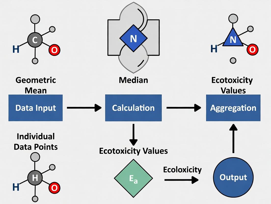
Diagram 1: From Data Variability to Informed Decision-Making
The Scientist's Toolkit: Essential Research Reagent Solutions
Table 3: Key Reagents, Organisms, and Tools for Ecotoxicity Research
| Item | Function & Description | Typical Use Case |
|---|---|---|
| Standard Test Organisms | Freshwater Algae (Raphidocelis subcapitata): Primary producer. Crustacean (Daphnia magna): Primary consumer. Fish (Danio rerio, fathead minnow): Vertebrate predator. | Constituting the base set for aquatic hazard assessment according to OECD guidelines [2]. |
| Reference Toxicants | Potassium dichromate, sodium chloride, copper sulfate. | Routine checking of organism health and sensitivity, ensuring laboratory consistency over time. |
| Solvent Carriers | Acetone, dimethyl sulfoxide (DMSO), ethanol. | Dissolving poorly water-soluble test chemicals, with concentration kept low (e.g., ≤0.1%) to avoid solvent toxicity. |
| Analytical Standards | Certified reference materials (CRMs) for target chemicals (e.g., PFOA, PFOS). | Verifying analytical method accuracy and quantifying measured vs. nominal concentration discrepancies [7]. |
| Data Aggregation Tools | Standartox R Package/Web App: Automates retrieval, filtering, and geometric mean aggregation of ecotoxicity data from ECOTOX [5]. | Deriving single, reproducible toxicity values for risk assessment and model input. |
| QSAR Prediction Tools | ECOSAR: Predicts toxicity based on chemical class. US EPA TEST: Estimates toxicity using multiple computational methodologies [6]. | Filling data gaps for chemicals lacking experimental values; used with caution due to varying predictive performance [9] [6]. |
| Curated Databases | ECOTOX Knowledgebase: Comprehensive repository of primary study results. REACH Database: High-quality study summaries submitted under EU regulation. CompTox/ToxValDB: Aggregates data from multiple public sources [5] [6]. | Sourcing experimental data for chemical assessments and meta-analyses. |
Advanced Models and Data Gap Filling
When experimental data are scarce, models provide essential estimates, though with limitations.
Machine Learning and QSARs
Machine learning models, such as random forest algorithms trained on chemical properties and mode of action, can estimate hazardous concentrations (HC50) for chemicals missing data in life cycle assessment (LCA) models like USEtox [9]. Such models can explain a significant portion of variability (R² ~0.63) and outperform traditional QSARs like ECOSAR in some cases [9]. However, a 2024 comparison showed that effect factors (EFs) calculated from estimated QSAR data (ECOSAR, TEST) correlated poorly with those derived from experimental data, underscoring the need for caution and transparency when using predicted values [6].
From Data to Policy: USEtox and Hazard Values
The USEtox model employs SSDs to calculate characterization factors for LCA. Research comparing hazard value derivation methods using REACH data found that:
- Chronic NOEC-equivalent data produced hazard values that aligned best with the EU's Classification, Labelling and Packaging (CLP) regulation [4].
- The commonly used acute-to-chronic extrapolation factor of 2 was found to be simplistic. Calculated geometric mean ratios were higher: 10.64 for fish, 10.90 for crustaceans, and 4.21 for algae [4].
- Reliance solely on acute EC50 data or the standard USEtox method may underestimate the number of chemicals classified as "very toxic to aquatic life" [4].
Diagram 2: Deriving an Effect Factor via Species Sensitivity Distribution
Table 4: Performance of Different Data Sources for Effect Factor Calculation [6]
| Data Source | Number of Substances with Calculated EFs | Correlation with USEtox Benchmark EFs | Key Advantage | Key Limitation |
|---|---|---|---|---|
| Experimental (REACH/CompTox) | 8,869 (added to 2,426 existing) | High | High confidence; based on measured biological effects. | Data unavailable for many thousands of chemicals. |
| QSAR (ECOSAR) | 6,029 | Low | Fills data gaps for organic chemicals; readily available. | High uncertainty; poor correlation with experimental benchmarks. |
| QSAR (US EPA TEST) | 6,762 | Low | Fills data gaps; uses consensus modeling. | High uncertainty; predictive performance varies by chemical class. |
Managing ecotoxicity data variability is a multi-step process requiring sound experimental design, rigorous data curation, and a justified statistical approach to aggregation. Based on the comparative analysis:
- Recommend the geometric mean over the median for aggregating multiple toxicity values for the same test combination. It makes better use of all data, is theoretically justifiable for log-normal distributions, and supports reproducible, consistent decision-making [1] [5].
- Implement robust experimental protocols, including adequate sample sizes (n>7/group where possible) [8] and measured concentration verification [7], to reduce variability at its source.
- Apply transparent data quality scoring (e.g., MCDA frameworks) before aggregation to weight or exclude unreliable data [3].
- Use estimated QSAR and machine learning data with clear caveats. They are essential for filling gaps but are not substitutes for high-quality experimental data [9] [6].
- Select hazard derivation methods aligned with assessment goals. For policy alignment, chronic NOEC-based values may be most appropriate, while the standard USEtox method provides consistency for comparative LCA [4].
The geometric mean, embedded within a workflow that prioritizes data quality and transparency, remains the most robust tool for navigating the inherent variability in ecotoxicity data and translating complex experimental results into actionable scientific insights and protective policies.
Mathematical Foundations and Core Properties
The geometric mean is a measure of central tendency, distinct from the arithmetic mean, that calculates the central value of a set of numbers by using the product of their values rather than their sum [10]. For a dataset of n positive values (𝑥₁, 𝑥₂, ..., 𝑥ₙ), the geometric mean is defined as the nth root of the product of all values [11]:
GM = (𝑥₁ · 𝑥₂ · ... · 𝑥ₙ)^(1/𝑛)
A key mathematical property is its relationship with logarithms. The geometric mean can be equivalently calculated by taking the exponential of the arithmetic mean of the natural logarithms of the values [10]:
GM = exp[(ln(𝑥₁) + ln(𝑥₂) + ... + ln(𝑥ₙ)) / 𝑛]
This logarithmic transformation is particularly useful for handling datasets with wide ranges or multiplicative relationships and helps avoid computational issues like arithmetic overflow [10].
- Inequality Relationship: For any dataset of positive numbers with at least one pair of unequal values, the harmonic mean is always the least of the three Pythagorean means, the arithmetic mean is always the greatest, and the geometric mean always lies between them [10]. Formally,
HM ≤ GM ≤ AM. - Minimization Property: The geometric mean is the minimizer of the sum of squared logarithmic deviations [10]. For a dataset, the value a that minimizes
∑ (log 𝑥ᵢ − log 𝑎)²is the geometric mean.
Diagram: Relationship Between Pythagorean Means
Comparative Analysis of Central Tendency Measures
The geometric mean exhibits distinct advantages and limitations compared to the arithmetic mean and median, especially in contexts relevant to toxicology, such as analyzing species sensitivity or chemical concentration data.
Table: Comparative Properties of Central Tendency Measures
| Property | Geometric Mean | Arithmetic Mean | Median |
|---|---|---|---|
| Mathematical Definition | nth root of the product of n values [10]. | Sum of values divided by n. | Middle value in an ordered list. |
| Data Relationship | Multiplicative [11]. | Additive. | Ordinal. |
| Sensitivity to Extreme Values | Less sensitive to high outliers (right-skew), but can be sensitive to values near zero. | Highly sensitive to extreme values (outliers). | Robust, insensitive to extreme values. |
| Typical Use Case in Ecotoxicology | Averaging log-normally distributed data (e.g., species sensitivity values, concentration ratios) [12]. Deriving HC50 in models like USEtox [13]. | Averaging normally distributed data. | Reporting typical value for highly skewed data or data with non-detects. |
| Data Requirement | All values must be positive ( >0 ) [14]. | Can handle positive and negative values. | No restriction on value sign. |
| Handling Zero Values | Cannot be calculated directly; requires adjustment (e.g., adding a constant). | Can be calculated. | Can be calculated. |
In ecological risk assessment, the geometric mean is often applied to aggregate toxicity data (e.g., multiple EC50 values for the same species-chemical pair) because species sensitivity distributions (SSDs) and many environmental concentration data are approximately lognormal [12]. This makes the geometric mean a more representative "average" than the arithmetic mean for such data. The median is favored when the dataset is small, contains non-detect values, or is highly skewed, as it provides a more robust central value unaffected by extreme outliers [12].
Role in Species Sensitivity Distribution (SSD) Modeling: Experimental Protocols
A primary application of the geometric mean in ecotoxicity research is within Species Sensitivity Distribution (SSD) modeling, a core method for deriving environmental safety thresholds like the Hazardous Concentration for 5% of species (HC5) [12].
Core SSD Workflow Protocol: This protocol is adapted from methodologies used to compare model-averaging and single-distribution approaches for HC5 estimation [12].
Data Curation and Geometric Mean Aggregation:
- Source: Collect acute (e.g., EC50, LC50) or chronic toxicity data from curated databases like EnviroTox [12] or U.S. EPA ECOTOX [15].
- Selection: Filter data based on reliability, relevance of endpoints, and water solubility limits (e.g., excluding concentrations >5x solubility) [12].
- Aggregation: For a given chemical, if multiple toxicity values exist for a single species, aggregate them using the geometric mean to obtain one representative value per species [12].
Reference HC5 Calculation (For Validation):
- For chemicals with large datasets (>50 species from diverse taxonomic groups), a reference HC5 can be calculated non-parametrically as the 5th percentile of the aggregated geometric mean values [12].
Subsampling Simulation:
- To simulate typical data-poor conditions, create subsampled datasets by randomly selecting toxicity data for 5-15 species from the full dataset [12].
SSD Fitting and HC5 Estimation:
- Fit parametric statistical distributions (e.g., log-normal, log-logistic, Burr Type III) to the log-transformed toxicity data from the subsample.
- Alternative Approach (Model Averaging): Fit multiple distributions and use a weighted average (based on goodness-of-fit criteria like AIC) of their HC5 estimates [12].
Performance Evaluation:
- Compare the HC5 estimates from the subsampled SSDs (from both single-distribution and model-averaging approaches) against the reference HC5. Assess performance by calculating the deviation or error [12].
Diagram: SSD-Based HC5 Estimation Workflow
Table: Key Findings from SSD Method Comparison Studies
| Method | Typical Input Data | Key Finding | Reference/Context |
|---|---|---|---|
| Single Distribution (Log-Normal) | Log-transformed EC50/LC50 values (geometric means per species). | HC5 estimates showed comparable precision to more complex model-averaging approaches in simulation tests [12]. | Iwasaki & Yanagihara (2025) comparison study [12]. |
| Model-Averaging (Multiple Distributions) | Log-transformed EC50/LC50 values (geometric means per species). | Did not guarantee reduced prediction error over single best-fit distribution; HC5 estimates could be insensitive to new data [12]. | Iwasaki & Yanagihara (2025) [12]. |
| Non-Parametric (Reference) | Full dataset of geometric mean toxicity values (>50 species). | Serves as a benchmark ("reference HC5") for validating parametric models under data-limited scenarios [12]. | Used for validation in methodological studies [12]. |
Computational and Predictive Modeling Applications
Beyond direct calculation, the geometric mean is foundational in computational tools for predicting ecotoxicity.
USEtox Effect Factors: In the life cycle assessment model USEtox, the geometric mean is central to calculating the ecotoxicity effect factor (EF). For a chemical, the hazardous concentration for 50% of species (HC50) is calculated as the arithmetic mean of the logarithmized geometric means of species-specific chronic toxicity values [13]. This log-transformed averaging is mathematically equivalent to the geometric mean of the geometric means, ensuring consistency with the expected log-normal distribution of species sensitivity.
Machine Learning for Data Gap Filling: Machine learning models are trained to predict HC50 or HC5 values using chemical descriptors. A 2023 study used a random forest model to estimate HC50 values for USEtox, achieving an average coefficient of determination (R²) of 0.630 on test sets [9]. The geometric mean of repeated experimental measurements for the same endpoint often forms the high-quality training data for such models [15] [6].
Table: Performance of Predictive Models in Ecotoxicity
| Model Type | Prediction Target | Key Performance Metric | Context & Implication |
|---|---|---|---|
| Random Forest (ML) | HC50 for characterization factors [9]. | Avg. Test Set R² = 0.630 [9]. | Outperformed traditional QSAR models (e.g., ECOSAR) in explaining variability [9]. Useful for filling data gaps. |
| Quantitative Structure-Activity Relationship (QSAR) | e.g., EC50 estimates from ECOSAR [6]. | Lower correlation with experimental USEtox factors vs. experimental data [6]. | Highlights caution needed when using estimated data; different QSAR tools can yield varied results [6]. |
| Global SSD Models | pHC5 for untested chemicals [15]. | Built on 3250 toxicity records across 14 taxonomic groups [15]. | Allows prioritization of high-toxicity chemicals from large inventories (e.g., 188 out of 8449) [15]. |
Table: Key Research Reagent Solutions and Databases for Ecotoxicity Aggregation
| Resource Name | Type | Primary Function in Ecotoxicity Research | Relevance to Geometric Mean |
|---|---|---|---|
| EnviroTox Database [12] | Curated Database | Provides quality-controlled acute and chronic ecotoxicity data for numerous chemicals and species. | Serves as a primary source for obtaining species-specific toxicity values, which are aggregated using the geometric mean for SSD modeling. |
| U.S. EPA ECOTOX Knowledgebase [15] | Comprehensive Database | A publicly available repository of single-chemical toxicity data for aquatic and terrestrial life. | Used to gather experimental toxicity endpoints for building and validating SSDs and machine learning models. |
| USEtox Model [13] | Consensus Model | The scientific consensus model for calculating characterization factors for human and ecotoxicity in life cycle assessment. | Its underlying methodology uses the geometric mean (via log-averaging) to derive the central effect factor (HC50) for chemicals. |
| OpenTox SSDM Platform [15] | Computational Tool | An open-access platform providing SSD modeling tools and data. | Facilitates the application of SSD modeling, where the geometric mean is a standard pre-processing step for per-species data. |
| REACH & CompTox Databases [6] | Regulatory & Research Databases | Large collections of experimental and predicted chemical property and toxicity data. | Sources for extracting ecotoxicity data to calculate effect factors, where intra-species data aggregation via geometric mean is often required. |
In ecotoxicity data aggregation, selecting the appropriate summary statistic is a foundational decision that directly impacts the robustness of risk assessments and regulatory conclusions. This analysis compares the mathematical properties of the median against its primary alternative, the geometric mean, within the context of contemporary research on species sensitivity distributions (SSDs) and life cycle impact assessment (LCIA). While the median is a familiar measure of central tendency, its performance relative to the geometric mean in handling the skewed, log-normal distributions typical of ecotoxicity data is a critical point of debate[reference:0]. This guide objectively compares these contenders, presenting experimental data and methodologies to inform researchers, scientists, and drug development professionals.
Mathematical Definitions and Core Properties
- Median: The middle value of an ordered dataset. It is the 50th percentile, effectively splitting the data into two equal halves.
- Geometric Mean: The n-th root of the product of n numbers ( ( \sqrt[n]{x1 \times x2 \times ... \times x_n} ) ). It is equivalent to the exponential of the arithmetic mean of the log-transformed data, making it the natural measure of central tendency for log-normally distributed data.
The fundamental difference lies in their treatment of data distribution: the median is based solely on data rank, while the geometric mean incorporates the magnitude of all values, giving it a direct algebraic relationship with multiplicative processes.
Comparative Properties Table
The following table summarizes the key mathematical and practical properties of common aggregation statistics in ecotoxicity.
| Property | Median | Geometric Mean | Arithmetic Mean | Minimum | Maximum |
|---|---|---|---|---|---|
| Definition | 50th percentile | n-th root of the product of n values | Sum of values divided by n | Smallest value | Largest value |
| Sensitivity to Outliers | Robust (ignores extreme values) | Moderately Robust (less sensitive than arithmetic mean) | Highly Sensitive | Not Applicable | Not Applicable |
| Suitability for Skewed Data | Good | Excellent (inherently for log-normal data)[reference:1] | Poor | Poor | Poor |
| Use in Small Datasets | Can be unreliable (ignores distribution tails)[reference:2] | Preferred over median for small n[reference:3] | Unreliable | Conservative (protective) | Worst-case |
| Data Requirements | Ordinal scale | Ratio scale (positive values only) | Interval scale | Any scale | Any scale |
| Primary Use in Ecotoxicity | Descriptive statistic | Standard for SSD aggregation[reference:4] | Rarely recommended | Deriving conservative thresholds | Identifying extreme values |
Experimental Evidence and Performance Data
Evidence from Standartox: Geometric Mean as the Standard
The Standartox database, which standardizes toxicity data from the US EPA ECOTOXicology Knowledgebase, explicitly advocates for the geometric mean. Its automated workflow aggregates multiple test results for a chemical-species combination by calculating the minimum, geometric mean, and maximum, but not the median[reference:5]. The rationale is that the geometric mean is less influenced by outliers than the arithmetic mean and, critically, is preferable to the median because "the median completely ignores the tails of the data distribution, making it unreliable for small data sets"[reference:6]. Validation showed that 91.9% of Standartox's geometric mean values lie within one order of magnitude of manually curated values from the Pesticide Properties DataBase (PPDB)[reference:7].
Quantitative Comparison in Acute-to-Chronic Extrapolation
A comparative study on deriving chemical ecotoxicity hazard values provides direct numerical comparison between the median and geometric mean. The research calculated acute-to-chronic ratios (ACRs) using REACH data, presenting both statistics side-by-side[reference:8]. The data, summarized below, show that the geometric mean is consistently lower than the median for these ratios, reflecting its reduced sensitivity to high outliers in the typically right-skewed data.
Table: Median vs. Geometric Mean of Acute-to-Chronic Ratios (ACRs) from REACH Data[reference:9]
| Taxon & Endpoint | n | Median | Geometric Mean |
|---|---|---|---|
| Fish (EC50eq to chronic EC50eq) | 96 | 2.64 | 3.74 |
| Crustacean (EC50eq to chronic EC50eq) | 389 | 4.58 | 5.45 |
| Fish (EC50eq to chronic NOECeq) | 322 | 8.93 | 10.64 |
| Crustacean (EC50eq to chronic NOECeq) | 876 | 8.77 | 10.90 |
| Algae (EC50eq to chronic NOECeq) | 2342 | 3.40 | 4.22 |
Contemporary Adoption in Life Cycle Assessment
Recent methodological advancements continue to solidify the geometric mean's role. A 2025 framework for calculating ecotoxicity effects in Life Cycle Assessment (LCA) utilized a geometric mean-based aggregation process, generating over 79,000 aggregated effect concentration datapoints at the species level[reference:10]. This approach is central to deriving extrapolation factors for models like USEtox, underscoring its acceptance as the standard for handling heterogeneous ecotoxicity data in regulatory and comparative impact contexts[reference:11].
Detailed Experimental Protocols
Protocol 1: Standartox Data Aggregation and Validation
- Data Source: Quarterly downloads of the US EPA ECOTOX database[reference:12].
- Harmonization: Filtering to common endpoints (e.g., EC50, NOEC) and unit standardization.
- Aggregation: For each chemical-organism combination, calculate the minimum, geometric mean, and maximum of all available test results. Outliers beyond 1.5×IQR are flagged but included[reference:13].
- Validation: Aggregated geometric means are compared to authoritative values from the PPDB and QSAR-based estimates from ChemProp. Agreement is measured as the percentage of values within one order of magnitude[reference:14].
Protocol 2: Deriving Acute-to-Chronic Ratios (ACRs) for Hazard Values
- Data Source: Ecotoxicity data from EU REACH registration dossiers[reference:15].
- Data Preparation: Extract acute EC50 and chronic NOEC (or EC50) values. Calculate ratio (acute/chronic) for each species-chemical data pair.
- Statistical Aggregation: For each taxon (fish, crustacean, algae), calculate descriptive statistics (n, min, max, median, geometric mean, percentiles) of the ratios, typically excluding ratios less than 1[reference:16].
- Hazard Value Calculation: Use the geometric mean of the ratios (or the median for comparison) as an extrapolation factor to convert acute data to chronic equivalents for use in Species Sensitivity Distributions (SSDs)[reference:17].
Visualizing Workflows and Key Concepts
Diagram 1: Standartox Data Aggregation Workflow
Diagram 2: Median vs. Geometric Mean Sensitivity
| Item | Function/Description | Relevance to Aggregation |
|---|---|---|
| US EPA ECOTOX KB | Comprehensive database of ecotoxicological test results. | Primary source of raw, multi-study data requiring aggregation. |
| REACH Dossiers | EU regulatory database with extensive submitted toxicity data. | Key source for deriving hazard values and extrapolation factors. |
| Standartox R Package | Tool for automated data download, harmonization, and geometric mean aggregation. | Implements the standardized workflow comparing min/geom/max. |
R with ssd packages |
Statistical environment (e.g., fitdistrplus, ssdtools). |
Used to fit Species Sensitivity Distributions (SSDs) based on aggregated geometric means. |
| USEtox Model | UNEP/SETAC consensus model for toxicity characterization in LCA. | End-user of aggregated ecotoxicity data (e.g., HC50 values) for impact assessment. |
| Geometric Mean Formula | ( \exp(\frac{1}{n}\sum{i=1}^{n} \ln(xi)) ) | The essential calculation for aggregating log-normal ecotoxicity data. |
The geometric mean emerges as the mathematically and practically superior contender for aggregating ecotoxicity data, particularly within the frameworks of SSDs and LCIA. Its property of dampening, rather than ignoring, the influence of extreme values makes it more reliable than the median for the typical small, skewed datasets in the field[reference:18]. Experimental evidence from standardization efforts like Standartox and contemporary research confirms its adoption as the benchmark method. While the median remains a useful descriptive statistic, its inability to incorporate information from the tails of the distribution limits its utility for deriving robust, reproducible aggregate values in ecotoxicological risk assessment and comparative guidance.
Within the context of geometric mean versus median ecotoxicity data aggregation research, a critical question persists: which measure offers greater robustness and sensitivity for deriving hazard values? This guide provides an objective, data-driven comparison of these two central tendency estimators, framing the discussion within the broader thesis on optimal data aggregation for species sensitivity distributions (SSDs) and life cycle impact assessment (LCIA).
Data Presentation: Quantitative Comparison of Aggregation Methods
The following table synthesizes key findings from recent studies comparing the geometric mean and the median in ecotoxicity data processing.
Table 1: Comparison of Geometric Mean and Median in Ecotoxicity Data Aggregation
| Study (Year) | Data Context | Key Finding Regarding Geometric Mean vs. Median | Quantitative Outcome (Where Available) | Source |
|---|---|---|---|---|
| GM-troph (2007) | HC50EC50 estimation for LCIA effect indicators. | The geometric mean is the most robust average estimator, especially for limited data (≤3 data points). The median was less favored. | Qualitative assessment based on theoretical and real-data tests. | [reference:0] |
| Standartox (2020) | Standardized aggregation of multiple ecotoxicity values for chemical-organism pairs. | The geometric mean is preferable over the median because the median "completely ignores the tails of the data distribution, making it unreliable for small data sets." | 91.9% of Standartox geometric mean values were within one order of magnitude of manually curated PPDB values (n=3601). | [reference:1][reference:2] |
| Saouter et al. (2019) | Acute-to-chronic extrapolation (ACE) ratios from EU REACH data. | Provides direct numerical comparison of median and geometric mean for ACE ratios across taxa. | Fish ACE ratios (n=96): Median = 2.64, Geometric Mean = 3.74. Crustacean ACE ratios (n=389): Median = 4.58, Geometric Mean = 5.45. | [reference:3] |
| Extrapolation Factors (2025) | Harmonization of ecotoxicity data for LCA. | The geometric mean-based aggregation process was used to produce tens of thousands of aggregated datapoints, facilitating derived extrapolation factors. | Process yielded 79,001 aggregated effect concentration datapoints at the species level. | [reference:4] |
Experimental Protocols
GM-troph Robustness Testing Protocol
The foundational GM-troph study established a methodology for comparing aggregation robustness[reference:5].
- Objective: To determine the most robust average estimator (arithmetic mean, geometric mean, or median) for the hazardous concentration for 50% of species (HC50EC50) under low-data conditions.
- Data: Real ecotoxicity effect data for eleven substances representing seven different toxic modes of action.
- Procedure:
- Data Subsampling: For each substance, multiple HC50EC50 values were simulated or derived from available species data.
- Aggregation Calculation: The arithmetic mean, geometric mean, and median were calculated for each subsample.
- Stability Assessment: The variability of each estimator was examined when the number of data points was limited (e.g., as few as three points, mirroring common LCIA data scarcity).
- Performance Evaluation: Estimators were ranked based on their statistical stability and resistance to bias from skewed data or outlier values.
- Outcome: The geometric mean demonstrated superior robustness, leading to its recommendation as the preferred estimator for HC50EC50 in LCIA[reference:6].
Standartox Data Aggregation Workflow
The Standartox tool implements a standardized pipeline for aggregating ecotoxicity data[reference:7].
- Objective: To automatically harmonize multiple ecotoxicity test results for a given chemical-organism combination into a single, reproducible aggregated value.
- Data Source: Quarterly releases of the US EPA ECOTOX knowledgebase.
- Procedure:
- Data Retrieval & Filtering: The pipeline downloads the ECOTOX database, and users can filter results based on taxonomic, chemical, and endpoint parameters.
- Outlier Flagging: Values exceeding 1.5 times the interquartile range are flagged (though not automatically excluded).
- Aggregation: For each unique chemical-organism-endpoint combination, the geometric mean of all available values is calculated. The minimum and maximum are also computed for context.
- Validation: Aggregated geometric means are compared to values from curated databases (e.g., PPDB) to assess accuracy, defined as falling within one order of magnitude.
- Rationale for Geometric Mean: This method was selected over the median due to its relative robustness against outliers and its incorporation of all data points, which is deemed critical for reliable aggregation, particularly with small datasets[reference:8].
Mandatory Visualization
Diagram 1: Ecotoxicity Data Aggregation & Comparison Workflow
This diagram outlines the logical workflow for processing ecotoxicity data and comparing the geometric mean and median estimators.
Diagram Title: Workflow for Comparing Geometric Mean and Median in Ecotoxicity
This table details key materials and digital resources essential for conducting research in ecotoxicity data aggregation.
Table 2: Key Research Reagent Solutions for Ecotoxicity Aggregation Studies
| Item / Resource | Function in Research | Example / Source |
|---|---|---|
| ECOTOX Knowledgebase | The primary public repository of curated aquatic and terrestrial ecotoxicity test results, serving as the fundamental data source for aggregation studies. | US EPA ECOTOX [reference:9] |
| Standartox Tool & R Package | Provides an automated, reproducible pipeline for downloading, filtering, and aggregating ECOTOX data using the geometric mean, enabling standardized analysis. | standartox R package [reference:10] |
| Model Test Organisms | Standard species used in toxicity testing, whose data forms the basis for aggregating chemical-specific sensitivity. | Daphnia magna (crustacean), Raphidocelis subcapitata (algae), Danio rerio (fish) [reference:11] |
| Statistical Software (R/Python) | Essential for implementing aggregation algorithms, calculating SSDs, and performing robustness simulations (e.g., bootstrap, Monte Carlo). | R with packages like fitdistrplus, ssd; Python with SciPy, pandas. |
| Reference Datasets (PPDB, EnviroTox) | Manually curated databases used as benchmarks to validate the accuracy and reliability of automated aggregation methods. | Pesticide Properties DataBase (PPDB), EnviroTox database [reference:12][reference:13] |
| SSD Fitting Tools | Software routines used to fit statistical distributions to aggregated toxicity data and derive protective concentrations (e.g., HC5). | R package ssd; web-based tools like the US EPA's SSD Generator. |
From Theory to Practice: Implementing Data Aggregation in Ecotoxicity Workflows
The foundation of robust ecotoxicity research lies in the quality and comparability of underlying data. The first critical step is sourcing and harmonizing raw toxicity information from large-scale repositories such as the US EPA's ECOTOX knowledgebase and the EU's REACH database. This process directly impacts downstream analyses, including the pivotal debate on whether to aggregate species-level data using the geometric mean or the median. This guide objectively compares leading tools and methodologies for this task, providing researchers with a clear framework for selecting the optimal approach for their work.
Comparison of Data Sourcing and Harmonization Tools
The landscape of ecotoxicity data resources varies widely in scope, automation, and aggregation philosophy. The following table summarizes key alternatives, with Standartox presented as a benchmark for automated, reproducible harmonization.
Table 1: Comparison of Ecotoxicity Data Resources and Harmonization Tools
| Tool / Database | Primary Data Source | Coverage (Approx.) | Aggregation Method | Key Validation / Performance Metric | Access & Usability |
|---|---|---|---|---|---|
| Standartox | ECOTOX (quarterly updates)[reference:0] | ~600,000 test results, ~8,000 chemicals, ~10,000 taxa[reference:1] | Geometric mean (preferred), min, max[reference:2] | 91.9% of aggregated values within one order of magnitude of PPDB reference values (n=3,601)[reference:3] | R package & web application; fully automated pipeline[reference:4] |
| ECOTOX Knowledgebase (Raw) | Primary literature & regulatory studies | ~1.1 million entries, >12,000 chemicals, ~14,000 species[reference:5] | None (raw data) | N/A | Web interface; bulk download available; requires manual curation |
| REACH Database (Raw) | Industry submissions under EU regulation | Initial: 305,068 records; Usable after QC: 54,353 records[reference:6] | None (raw data) | ~82% of initial data excluded due to quality/reporting issues[reference:7] | ECHA portal; complex structure; requires significant cleaning[reference:8] |
| EnviroTox Database | ECOTOX & other sources | Limited to aquatic organisms (fish, amphibians, invertebrates, algae)[reference:9] | Rule-based algorithm for single toxicity value per taxon[reference:10] | N/A (focused on quality-controlled values for aquatic SSDs) | Curated dataset; less taxonomic breadth than Standartox[reference:11] |
| PPDB (Pesticides Properties DB) | Literature & regulatory data | ~2,000 pesticides[reference:12] | Manual expert judgment for single values per species[reference:13] | Used as a quality benchmark for other tools[reference:14] | Focused resource for pesticides only; not automated |
Experimental Protocols for Aggregation Validation
The superiority of a harmonization tool is demonstrated through rigorous validation against independent benchmarks. The following protocols detail key experiments that quantitatively assess performance.
- Objective: To assess the accuracy of Standartox's automated geometric mean aggregation against manually curated reference values.
- Data Source: Standartox aggregated values and corresponding ecotoxicity data for the same chemical-species combinations from the Pesticide Properties Database (PPDB)[reference:15].
- Methodology:
- Overlapping chemical-species records between Standartox and PPDB were identified (n=3,601).
- For each record, the Standartox geometric mean value was compared to the PPDB reference value.
- The comparison metric was the percentage of Standartox values lying within one order of magnitude (i.e., a factor of 10) of the PPDB value[reference:16].
- Outcome: 91.9% of Standartox aggregated values met the acceptance criterion, validating the automated pipeline's reliability[reference:17].
Protocol 2: Comparison with QSAR Model Predictions (ChemProp)
- Objective: To evaluate the consistency of harmonized experimental data with in silico predictions.
- Data Source: Standartox geometric mean LC50 values for Daphnia magna and predicted LC50 values from the QSAR software ChemProp[reference:18].
- Methodology:
- Daphnia magna LC50 data were extracted from Standartox.
- Corresponding predictions were obtained from ChemProp for the same chemicals (n=179).
- Agreement was measured as the percentage of Standartox values within one order of magnitude of the ChemProp prediction[reference:19].
- Outcome: 95% of Standartox values were within one order of magnitude of ChemProp predictions, demonstrating alignment between harmonized experimental data and computational models[reference:20].
Protocol 3: Geometric Mean vs. Median Aggregation
- Objective: To empirically justify the choice of geometric mean over median for species-level aggregation, a core thesis in ecotoxicity data analysis.
- Data Source: Multi-test data for chemical-species combinations within the ECOTOX database.
- Methodology:
- For a given chemical and species, all available toxicity values (e.g., EC50) are collected.
- Both the geometric mean and the median are calculated for the dataset.
- The robustness and representativeness of each statistic are evaluated, particularly for small sample sizes where the median's ignorance of distribution tails is a critical flaw[reference:21].
- Theoretical Basis: The geometric mean is less influenced by outliers than the arithmetic mean and, crucially, incorporates information from the entire data distribution (including tails), unlike the median. This makes it more reliable for deriving representative toxicity values, especially with limited data[reference:22].
Visualizing Workflows and Methodologies
Diagram 1: Ecotoxicity Data Harmonization Pipeline
This diagram outlines the generalized workflow for sourcing raw data from major repositories and processing it into a harmonized, analysis-ready format.
Diagram 2: Geometric Mean vs. Median Aggregation Logic
This diagram contrasts the underlying logic of the two primary aggregation methods within the context of species sensitivity data.
Successfully executing data sourcing and harmonization requires a combination of software tools, data resources, and methodological knowledge.
Table 2: Essential Toolkit for Ecotoxicity Data Harmonization Research
| Category | Item | Function / Purpose | Example / Note |
|---|---|---|---|
| Core Software | R Programming Environment | Provides the statistical foundation and scripting capability for reproducible data cleaning, analysis, and automation[reference:24]. | Essential for running packages like standartox. |
| Standartox R Package / API | Enables programmatic access to the pre-harmonized Standartox database and its aggregation functions[reference:25]. | Facilitates integration into custom analysis workflows. | |
| Primary Data Sources | EPA ECOTOX Knowledgebase | The largest public repository of curated ecotoxicity test results, serving as the primary input for many harmonization tools[reference:26]. | Downloaded quarterly for updates. |
| ECHA REACH Database | A vast source of regulatory ecotoxicity data for chemicals in the EU market, requiring extensive processing to be usable[reference:27]. | Useful for regulatory alignment studies. | |
| Reference & Validation | PPDB (Pesticide Properties DB) | A manually curated database providing high-quality reference values for pesticide toxicity, used as a validation benchmark[reference:28]. | Serves as a "gold standard" for validation protocols. |
| QSAR Software (e.g., ChemProp) | Provides in silico toxicity predictions used to compare against and complement harmonized experimental data[reference:29]. | Helps assess data plausibility and fill gaps. | |
| Methodological Guidance | Species Sensitivity Distribution (SSD) Theory | The conceptual framework for aggregating species-level data to estimate hazardous concentrations (HCx) for ecosystems. | Underpins the use of geometric mean aggregation. |
| Geometric Mean Aggregation Protocol | The standardized statistical method for deriving a single representative toxicity value from multiple tests, preferred over median[reference:30]. | A critical step in the harmonization pipeline. |
The derivation of robust environmental safety thresholds, such as Predicted-No-Effect Concentrations (PNECs) or Environmental Quality Standards (EQS), fundamentally relies on the aggregation of ecotoxicity data [16]. Within the research context of comparing geometric mean versus median aggregation methods for species sensitivity distributions (SSDs), the initial step of applying stringent quality filters is not merely preparatory—it is determinative. The choice between geometric mean and median for summarizing multiple toxicity values for a single species-chemical combination, or for estimating hazardous concentrations (e.g., HC5) from an SSD, is secondary to the foundational quality of the input data [12].
Inconsistent or biased reliability evaluations can directly alter the dataset used for aggregation, thereby influencing the final hazard assessment and potentially leading to underestimated environmental risks or unnecessary mitigation costs [17]. This guide objectively compares the predominant quality evaluation frameworks—the established Klimisch method and the modern CRED (Criteria for Reporting and Evaluating Ecotoxicity Data) criteria. It details their application, supported by experimental ring-test data, to provide researchers and risk assessors with a clear basis for selecting a method that ensures transparency, consistency, and scientific rigor in the data foundation upon which all subsequent aggregation decisions are made [16] [17].
Comparative Analysis of Klimisch and CRED Evaluation Frameworks
The Klimisch method, developed in 1997, has been a regulatory cornerstone for evaluating study reliability but has faced criticism for its lack of detail and guidance [17]. The CRED method was developed to address these shortcomings, providing a more structured and transparent framework [16].
Table 1: Core Structural Comparison of the Klimisch and CRED Evaluation Methods
| Feature | Klimisch Method (1997) | CRED Method (2016) |
|---|---|---|
| Primary Scope | Reliability evaluation only. | Combined evaluation of Reliability (20 criteria) and Relevance (13 criteria) [16] [17]. |
| Reliability Categories | 4-point scale: Reliable without restrictions (R1), Reliable with restrictions (R2), Not reliable (R3), Not assignable (R4) [17]. | Detailed criteria-based evaluation leading to the same 4-category conclusion, but with explicit, guided justification [17]. |
| Relevance Evaluation | No formal criteria or categories provided [17]. | Formal criteria and 3 categories: Relevant without restrictions (C1), Relevant with restrictions (C2), Not relevant (C3) [16] [17]. |
| Guidance & Specificity | Limited, high-level criteria. Lacks detailed guidance, leaving significant room for expert judgment [16]. | Extensive guidance for each criterion, reducing ambiguity. Includes specific reporting recommendations for authors [16]. |
| Bias Consideration | Criticized for potential bias towards industry-sponsored Guideline/GLP studies, potentially overlooking valid non-standard research [16] [17]. | Designed for neutral application to all studies, whether guideline or peer-reviewed literature, based solely on scientific merit [17]. |
| Tool Format | Descriptive text. | Supported by structured Excel tools for systematic evaluation and documentation [18] [19]. |
Experimental Data and Performance Comparison
A pivotal international ring test involving 75 risk assessors from 12 countries was conducted to directly compare the two methods [17]. Participants evaluated aquatic ecotoxicity studies using both frameworks. The results quantitatively demonstrate CRED's advantages in consistency and transparency.
Table 2: Quantitative Ring-Test Results Comparing Evaluation Consistency [17]
| Evaluation Aspect | Klimisch Method Performance | CRED Method Performance | Implication |
|---|---|---|---|
| Inter-assessor Consistency (Reliability) | Low. Assessments for the same study frequently spanned multiple categories (e.g., R1 to R3). | High. Majority consensus on the final reliability category was significantly more frequent. | CRED reduces arbitrariness, leading to more reproducible hazard identification. |
| Handling of Relevance | Not systematically addressed, leading to inconsistent consideration of study fitness-for-purpose. | Enabled structured, purpose-driven evaluation, improving alignment between data and assessment goals. | Ensures aggregated data (e.g., for SSDs) is appropriate for the specific regulatory context. |
| Perceived Dependence on Expert Judgment | Rated as high by participants. | Rated as substantially lower. | Promotes objectivity and reduces the potential for evaluator bias in the data screening phase. |
| Perceived Transparency | Rated as low; evaluation rationale often opaque. | Rated as high due to requirement for criterion-specific documentation. | Creates an audit trail, crucial for defending data choices in geometric mean vs. median aggregation research. |
| Time Requirement | Perceived as faster due to simplicity. | Perceived as slightly more time-consuming but worthwhile due to increased rigor and reduced need for re-evaluation. | Initial investment in quality filtering saves time during later data analysis and dispute resolution. |
Detailed Experimental Protocol: The CRED vs. Klimisch Ring Test
The methodology of the comparative ring test provides a model for validating quality assessment frameworks [17].
- Phase 1 (Klimisch Evaluation): Each participant evaluated the reliability and (where possible) relevance of two out of eight preselected aquatic ecotoxicity studies using the Klimisch method. Relevance was summarized ad-hoc using three categories (C1-C3).
- Phase 2 (CRED Evaluation): Each participant evaluated two different studies from the same set using a draft version of the CRED Excel tool, which included specific criteria for both reliability and relevance.
- Study Design: To ensure independence, the studies evaluated in Phases 1 and 2 were different, and participants from the same institute did not evaluate the same study.
- Contextualization: Participants were instructed to evaluate studies for the purpose of deriving Environmental Quality Criteria under the EU Water Framework Directive, standardizing the relevance perspective [17].
- Data Collection: After each phase, participants completed a questionnaire assessing the method's practicality, their confidence in the evaluation, and any missing criteria.
- Analysis: Consistency was measured by the degree of consensus on the final reliability/relevance category for each study under each method. Questionnaire responses were analyzed thematically.
Integration with Data Aggregation Research: From Filtered Data to SSDs
Applying rigorous quality filters via CRED directly impacts downstream aggregation research. A dataset curated with CRED will consist of studies where experimental conditions, statistical reporting, and biological relevance are clearly documented and validated [16]. This high-quality input is essential for robust SSD modeling, where the choice between parametric (e.g., log-normal, log-logistic) and non-parametric approaches, or between using geometric means versus medians for intra-species data, becomes a purely statistical decision rather than one confounded by data quality issues [12].
Recent research on SSD modeling confirms that with a sufficient number of high-quality, reliable data points, the choice of statistical distribution (e.g., for model averaging vs. a single-distribution approach) has a more nuanced impact on the HC5 estimate than the underlying data quality itself [12]. Furthermore, computational toxicology frameworks that integrate heterogeneous biological data (e.g., knowledge graphs linking chemicals to genes and pathways) for toxicity prediction depend on reliable experimental data for training and validation, underscoring the foundational role of quality evaluation across traditional and New Approach Methodologies (NAMs) [20].
Title: Workflow for Quality Filtering in Ecotoxicity Data Aggregation Research
The Scientist's Toolkit: Essential Research Reagent Solutions
Table 3: Key Research Tools and Resources for Quality Evaluation and Data Aggregation
| Tool/Resource | Function in Research | Relevance to Aggregation Studies |
|---|---|---|
| CRED Excel Evaluation Tool [18] [19] | Provides a standardized worksheet to systematically score the 20 reliability and 13 relevance criteria for an ecotoxicity study. | Ensures transparent, documented quality filtering, creating a defensible curated dataset for geometric mean/median comparisons. |
| EnviroTox Database [12] | A curated database of ecotoxicity studies with pre-applied quality filters (e.g., excluding data above water solubility). | A primary source for high-quality, pre-screened toxicity data used in SSD modeling and aggregation method research. |
| OpenTox SSDM Platform [15] | An open-access platform for building and analyzing Species Sensitivity Distribution models. | Enables testing of how different data aggregation methods (e.g., geometric mean input) affect HC5 estimates across statistical models. |
| Toxicological Knowledge Graph (ToxKG) [20] | A structured database integrating chemicals, genes, pathways, and assay data to inform mechanistic toxicity. | Provides biological context which can help assess the relevance of studies for specific modes of action, influencing data inclusion for aggregation. |
| CREED for Exposure Data [21] | A sister framework to CRED for evaluating the reliability and relevance of environmental monitoring (exposure) datasets. | Critical for the complementary exposure side of risk assessment, ensuring high-quality concentration data for risk quotient calculations. |
Title: Logical Framework: Quality Filtering's Role in Data Aggregation Research
The comparative analysis demonstrates that the CRED evaluation method offers a superior framework for applying quality filters in ecotoxicity research compared to the traditional Klimisch method. Its structured criteria, explicit guidance, and proven higher consistency make it the recommended choice for constructing datasets intended for advanced aggregation research, such as comparing geometric mean and median approaches.
For researchers focused on data aggregation methodologies, the following application pathway is recommended:
- Primary Filtering: Employ the CRED criteria as the primary quality filter to build a foundation dataset. The Excel tool facilitates transparent documentation [19].
- Contextual Relevance: Clearly define the assessment purpose (e.g., derivation of chronic PNEC for a specific mode of action) when applying relevance criteria to ensure aggregated data is fit-for-purpose [16].
- Aggregation on Clean Data: Conduct geometric mean vs. median comparisons using the data curated through CRED. This isolates the statistical question from data quality confounders.
- Sensitivity Analysis: Perform sensitivity analyses to determine how the inclusion of studies rated "reliable/relevant with restrictions" under CRED affects the outcomes of different aggregation methods.
By adopting the CRED framework, the research community can ensure that the ongoing scientific discourse on optimal data aggregation techniques is built upon a consistent, transparent, and high-quality data foundation, ultimately leading to more reliable environmental safety standards.
Within the broader research on geometric mean vs. median ecotoxicity data aggregation, executing the geometric mean is a critical, non-negotiable step for deriving robust hazard values. Aggregation reduces multiple toxicity data points for a single chemical and species to a singular, representative value, which forms the foundation for higher-order calculations like Species Sensitivity Distributions (SSDs) and Hazardous Concentrations (HCp) [12]. The choice of aggregation method directly influences the outcome of environmental risk assessments and life cycle impact evaluations [4] [5].
While the median is a measure of central tendency less sensitive to outliers, the geometric mean is the established standard in ecotoxicology [5]. It is preferred because toxicity data are typically log-normally distributed, and the geometric mean provides a more accurate central value for multiplicative processes. Critically, for small datasets, the median can be unreliable as it ignores the distribution's tails, whereas the geometric mean incorporates all data points while dampening the influence of extreme values [5]. This guide provides a detailed, procedural framework for correctly executing geometric mean aggregation within contemporary research and regulatory workflows.
Foundational Principles and Comparative Framework
Rationale for Geometric Mean over Arithmetic Mean and Median
The geometric mean is defined as the nth root of the product of n numbers. Its application in ecotoxicology is justified by several key principles [22] [5]:
- Log-Normal Data: Species sensitivity to chemicals and the distribution of repeated toxicity tests for the same endpoint often follow a log-normal distribution. The geometric mean accurately reflects the central tendency of such data.
- Robustness to Skew: It is less influenced by exceptionally high or low outlier values compared to the arithmetic mean, providing a more conservative and stable estimate.
- Multiplicative Processes: Toxicological effects often relate to concentrations in a multiplicative manner (e.g., dose-response), making the geometric mean a mathematically appropriate descriptor.
A comparison of central tendency measures is summarized in the table below.
Table 1: Comparison of Central Tendency Measures for Ecotoxicity Data Aggregation
| Measure | Calculation | Best Use Case | Sensitivity to Outliers | Suitability for SSDs |
|---|---|---|---|---|
| Geometric Mean | (Π xᵢ)^(1/n) | Log-normally distributed data (standard for toxicity values) | Low | High (Recommended) [5] |
| Arithmetic Mean | (Σ xᵢ)/n | Normally distributed data | High | Low (Can overestimate safe levels) |
| Median | Middle value of ordered dataset | Data with severe, non-physical outliers | Very Low | Low for small datasets (ignores distribution tails) [5] |
Quantitative Basis from Major Databases
Large-scale analyses of regulatory data provide the empirical foundation for using geometric means. Key studies have calculated critical toxicity ratios using geometric mean aggregation [4] [23]:
- Analysis of the EU REACH database derived acute-to-chronic ratios for major taxonomic groups: 10.64 for fish, 10.90 for crustaceans, and 4.21 for algae [4].
- A 2025 study harmonizing data from REACH and CompTox databases used geometric mean aggregation to produce 79,001 species-level effect concentration datapoints for 10,668 chemicals, which were subsequently used to derive extrapolation factors [23].
- The Standartox database and tool automates the aggregation of ecotoxicity data from the US EPA ECOTOX knowledgebase, using the geometric mean as its primary aggregation method to produce standardized, reproducible toxicity values for chemical risk assessment [5].
Step-by-Step Protocol for Geometric Mean Aggregation
The following workflow details the standardized procedure for calculating a geometric mean value from a set of ecotoxicity data. This protocol aligns with methodologies employed by major databases and research initiatives [23] [6] [5].
Protocol Title: Geometric Mean Aggregation for Ecotoxicity Data
Objective: To aggregate multiple ecotoxicity test results (e.g., EC50, NOEC) for a specific chemical, species, and endpoint into a single, robust representative value using the geometric mean.
Materials:
- Dataset of curated ecotoxicity test results.
- Statistical software (e.g., R, Python) or calculation tool.
Procedure:
- Data Grouping: Assemble all valid test results for the identical combination of chemical, species, and toxicological endpoint (e.g., Daphnia magna 48-hour EC50 for Chemical X) [5].
- Log-Transformation: Convert each concentration value ((xi)) in the group to its base-10 logarithm ((yi = \log{10}(xi))). This stabilizes variance and normalizes skewed data.
- Calculate Mean of Logs: Compute the arithmetic mean ((\bar{y})) of the log-transformed values: (\bar{y} = \frac{\sum{i=1}^{n} yi}{n}), where (n) is the number of data points.
- Back-Transformation: Calculate the geometric mean (GM) by back-transforming the result: (GM = 10^{\bar{y}}).
- Optional - Robustness Check: Identify potential outliers using the Interquartile Range (IQR) method on the log-transformed data. Values exceeding (Q1 - 1.5 \times IQR) or (Q3 + 1.5 \times IQR) can be flagged for review [5]. (Note: Expert judgment is required for exclusion; the geometric mean is often calculated including flagged points due to its inherent robustness [5]).
Example Calculation: For three Daphnia magna EC50 values: 1.0 mg/L, 2.2 mg/L, and 5.1 mg/L.
- Log-transformed: 0.000, 0.342, 0.708.
- Arithmetic mean of logs: (0.000 + 0.342 + 0.708) / 3 = 0.350.
- Geometric Mean: (10^{0.350} = 2.24) mg/L.
Decision Protocol for Data Inclusion/Exclusion
A critical pre-aggregation step is determining which data points to include. There is no universal regulatory guideline for this [22]. The following decision logic, synthesized from current practice, should be applied during the data curation phase (Step 1 of the workflow).
Experimental Validation & Comparative Performance
Validation in Species Sensitivity Distribution (SSD) Estimation
The geometric mean's performance is validated in advanced SSD modeling. A 2025 study comparing SSD estimation methods used the geometric mean to aggregate multiple toxicity values for a single species before fitting distributions [12]. The study, analyzing 35 chemicals with extensive data (>50 species), found that SSD-derived hazardous concentrations (HC5) were reliable when based on geometric mean-aggregated inputs. This supports its use as a precursor step to community-level risk estimation [12].
Comparison with Model-Averaging and QSAR Data
Geometric mean aggregation also serves as a benchmark for evaluating predictive data.
- Model-Averaging SSDs: Research indicates that HC5 estimates from SSDs based on geometric mean-aggregated data show comparable precision to those from more complex model-averaging approaches that combine multiple statistical distributions [12].
- QSAR Prediction Aggregation: When using Quantitative Structure-Activity Relationship (QSAR) models like ECOSAR, which generate multiple predictions per chemical, the geometric mean is a standard method to derive a single point estimate. One large-scale study calculated the geometric mean of all applicable QSAR model outputs for a chemical to produce a consolidated prediction for use in hazard assessment [24].
Table 2: Application of Geometric Mean in Key Ecotoxicological Contexts
| Context | Data Input | Aggregation Action | Purpose & Outcome | Supporting Study |
|---|---|---|---|---|
| SSD Development | Multiple EC50/LC50 values for one species & chemical. | Compute species mean acute value (SMAV) as the geometric mean. | Creates the data points for fitting the SSD curve to estimate HC5. | [12] |
| Database Curation (e.g., Standartox) | All test results for a chemical-species-endpoint from ECOTOX. | Outputs the geometric mean as the standard aggregated value. | Provides reproducible, single toxicity values for risk indicators. | [5] |
| Extrapolation Factor Derivation | Paired acute-chronic data for many chemicals. | Calculate the geometric mean of acute:chronic ratios. | Derives generic assessment factors (e.g., acute-to-chronic ratio = 10). | [4] [23] |
| QSAR Prediction Reconciliation | Multiple model predictions from different QSAR classes. | Calculate geometric mean of all valid predictions. | Provides a consensus, single-point estimate from in silico tools. | [6] [24] |
The Scientist's Toolkit: Research Reagent Solutions
Implementing geometric mean aggregation requires access to curated data and specialized tools. The following toolkit lists essential resources for researchers.
Table 3: Research Reagent Solutions for Ecotoxicity Data Aggregation
| Item / Resource | Type | Primary Function in Aggregation | Key Reference / Source |
|---|---|---|---|
| Standartox Database & R Package | Software Tool / Database | Automates the curation, filtering, and geometric mean aggregation of ecotoxicity data from the EPA ECOTOX database. | [5] |
| REACH Ecotoxicity Database | Regulatory Database | Source of high-volume, curated experimental data for deriving aggregated hazard values and extrapolation factors. | [4] [23] |
| US EPA ECOTOX Knowledgebase | Comprehensive Database | Primary source of empirical ecotoxicity test results for tools like Standartox. Provides raw data for aggregation. | [5] [24] |
| CompTox Chemicals Dashboard | Integrated Database | Source of experimental toxicity data (via ToxValDB) used alongside REACH data for large-scale harmonization and factor derivation. | [23] [6] |
| R or Python Statistical Environment | Programming Language | Platform for executing custom data curation, log-transformation, and geometric mean calculation scripts. Essential for reproducible research. | Common Practice |
| USEtox Model & Database | Consensus Model | Uses aggregated chronic EC50 values (often derived via geometric mean) to calculate characterization factors for life cycle assessment. | [9] [6] |
| ECOSAR, VEGA, TEST | QSAR Software | Generate predicted toxicity values. Outputs from multiple models are often aggregated via geometric mean to fill data gaps. | [6] [24] |
Executing the geometric mean is a foundational, technically defined step in ecotoxicity data aggregation. Its superiority over the median and arithmetic mean for log-normal toxicity data is well-supported by theory and large-scale empirical practice [4] [5]. The protocol outlined here—encompassing data curation, log-transformation, and back-calculation—provides a standardized workflow that aligns with methods used by major regulatory databases and research consortia [23] [12] [5].
The resulting aggregated values are not an endpoint but a critical input for higher-order decision-making models, including SSDs for environmental quality standard setting and USEtox for comparative life cycle assessment. Mastery of this step ensures that subsequent assessments of chemical hazard and environmental risk are built upon a robust and representative foundation.
Within the broader research on geometric mean versus median aggregation for ecotoxicity data, the derivation of Species Sensitivity Distributions (SSDs) and Hazard Concentrations (HCs) represents the critical translational step. This phase transforms aggregated, chemical-specific toxicity values (e.g., geometric mean EC50 for a species) into robust, ecosystem-level estimates of risk [5]. SSDs model the variation in sensitivity among species, allowing regulators and scientists to determine concentrations predicted to affect a specified percentage (e.g., 5% or 20%) of species—the HC5 or HC20 [12] [23]. The choice of data aggregation method (geometric mean vs. median) directly influences the input values for SSD construction, thereby propagating uncertainty or robustness into these final protective benchmarks. This guide compares the performance of contemporary approaches for building SSDs and deriving HCs, framing them within the ongoing methodological evolution from simple distribution fitting to model-averaging and machine-learning-assisted techniques.
Performance Comparison of SSD and Hazard Concentration Derivation Methods
The selection of methodology for constructing SSDs significantly impacts the resulting hazard concentration estimates. The table below compares the core performance metrics, data requirements, and optimal use cases for the primary contemporary approaches.
Table: Comparison of Methods for Deriving Species Sensitivity Distributions (SSDs) and Hazard Concentrations (HCs)
| Method | Core Description | Key Performance Metrics | Data Requirements | Best Suited For |
|---|---|---|---|---|
| Single Parametric Distribution (e.g., Log-Normal) [12] | Fits a single statistical distribution (e.g., log-normal, log-logistic) to aggregated species sensitivity data to estimate the HC5. | Accuracy: Can produce large deviations from reference HC5 with limited data (<15 species) [12]. Precision: Comparable to model-averaging when using log-normal/log-logistic distributions [12]. Simplicity: Straightforward to implement and interpret. | Minimum of ~8-10 species from multiple taxonomic groups recommended; performance improves with >15 species [12]. | Initial screening, assessments with well-established data where a suitable distribution is known. |
| Model-Averaging Approach [12] | Fits multiple statistical distributions, weights them by goodness-of-fit (e.g., AIC), and calculates a weighted-average HC estimate. | Accuracy: Does not guarantee reduced error compared to single-distribution approach; deviations comparable to log-normal/log-logistic [12]. Robustness: Incorporates model selection uncertainty, making HC estimates less sensitive to adding new data points [12]. | Requires sufficient data to fit multiple models reliably; benefits from >10 species [12]. | Regulatory applications seeking conservative, stable estimates that account for model uncertainty. |
| Non-Parametric / Direct Percentile [12] | Directly calculates the HC5 as the 5th percentile of the empirical distribution of aggregated toxicity data. | Accuracy: Provides a direct "reference" HC5 when extensive data are available [12]. Bias: Unreliable with small datasets (<15-20 species) [12]. | Requires large datasets (>50 species) for a reliable estimate [12]. | Validation of parametric methods or assessments for chemicals with exceptionally rich toxicity datasets. |
| Machine Learning (ML)-Predicted HC50 [9] | Uses ML models (e.g., Random Forest) trained on chemical properties to directly predict the Hazardous Concentration for 50% of species (HC50). | Predictive Power: Random Forest models can explain ~63% (R²=0.630) of variability in USEtox HC50 [9]. Coverage: Can generate estimates for thousands of data-poor chemicals [9] [6]. Speed: Enables rapid screening. | Requires a training set of chemicals with known HC50 and associated physicochemical property data [9]. | Life Cycle Assessment (LCA) and high-throughput screening where effect factors for many chemicals are needed [9] [6]. |
| QSAR-Estimated Inputs for SSD [6] | Uses Quantitative Structure-Activity Relationship models to predict base toxicity endpoints (e.g., fish LC50), which are then aggregated and used in SSD construction. | Confidence: Low correlation with experimental data-based effect factors; high uncertainty [6]. Coverage: Provides data for otherwise data-less chemicals (e.g., ECOSAR covered 6029 chemicals) [6]. | Dependent on the applicability domain and quality of the QSAR model. | Filling data gaps for preliminary or prioritization assessments, with clear acknowledgment of uncertainty. |
Detailed Experimental Protocols
Protocol for Comparing Model-Averaging and Single-Distribution SSD Approaches
This protocol, based on a 2025 study, provides a framework for empirically evaluating HC estimation methods [12].
- Reference Dataset Curation: Select chemicals with acute toxicity data (EC50/LC50) for >50 species from at least three taxonomic groups (e.g., algae, invertebrates, fish). Use a quality-controlled database like EnviroTox [12].
- Reference HC5 Calculation: For each chemical, compute a reference HC5 as the 5th percentile of the complete, aggregated dataset (geometric mean per species) [12].
- Subsampling Simulation: To simulate typical data-poor conditions, randomly subsample species data from the complete set at various sample sizes (e.g., n = 5, 10, 15 species). Repeat this process multiple times (e.g., 1000 iterations) to account for variability [12].
- SSD Fitting and HC Estimation:
- Single-Distribution: Fit a log-normal distribution to each subsample and estimate the HC5 [12].
- Model-Averaging: Fit a set of distributions (e.g., log-normal, log-logistic, Weibull, Burr Type III) to each subsample. Use the Akaike Information Criterion (AIC) to calculate model weights and derive a weighted-average HC5 [12].
- Performance Evaluation: For each method and sample size, calculate the deviation (e.g., log difference) between the estimated HC5s from the subsamples and the reference HC5. Compare the accuracy and precision of the methods across all iterations [12].
Protocol for Data Harmonization and Aggregation for USEtox Factor Calculation
This protocol outlines the steps to create aggregated, harmonized inputs for SSD and effect factor calculation in LCA [23] [6].
- Raw Data Collection: Gather ecotoxicity data from major databases (e.g., US EPA CompTox, REACH dossiers, ECOTOX). Include endpoint, species, duration, and concentration type [23] [6].
- Data Cleaning and Standardization:
- Filter to relevant endpoints (e.g., EC50, NOEC, EC10).
- Standardize units and effect concentration indicators.
- Apply reliability criteria (e.g., exclude concentrations exceeding water solubility) [12].
- Data Aggregation:
- Extrapolation (if needed): Apply extrapolation factors to convert data to a consistent endpoint (e.g., chronic EC10). Use species group-specific factors where available for greater accuracy [23].
- SSD Construction and HC/EF Derivation: Use the aggregated dataset to fit an SSD (choosing an appropriate method from Section 2) and calculate the desired hazardous concentration (HC5 or HC20). For USEtox, the Effect Factor (EF) is calculated as 0.5 / HC50 [9] [6].
Visualizing the Workflow: From Aggregated Data to Hazard Concentrations
The following diagram maps the logical workflow and decision points involved in progressing from aggregated ecotoxicity data to final hazard concentrations.
Table: Essential Research Tools for SSD and Hazard Concentration Derivation
| Tool / Resource Name | Type | Primary Function in Research | Key Features / Notes |
|---|---|---|---|
| EnviroTox Database [12] | Curated Ecotoxicity Database | Provides quality-controlled, aggregated ecotoxicity data for SSD development. | Includes data for many species; used for method validation and reference HC derivation [12]. |
| US EPA CompTox Dashboard [9] [23] | Integrated Chemical Database | Source of physicochemical properties for ML models and raw toxicity data for harmonization. | Links chemical structures, properties, and experimental toxicity data from multiple sources [23]. |
| REACH Registration Dossiers [23] [6] | Regulatory Data Source | Provides extensive, often unpublished, ecotoxicity study results for data harmonization. | A critical source for experimental data, especially for industrial chemicals [6]. |
| Standartox Tool & Database [5] | Data Aggregation Tool | Automates the curation, filtering, and geometric mean aggregation of ECOTOX data. | Enables reproducible derivation of single toxicity values per species-chemical combination [5]. |
| USEtox Model [9] [23] [6] | Consensus LCIA Model | The standard framework for calculating ecotoxicity characterization factors, requiring HC50/EF as input. | The primary application driver for many HC derivation efforts in lifecycle assessment [6]. |
R packages (e.g., fitdistrplus, ssdtools) |
Statistical Software | Facilitates the fitting of multiple statistical distributions to data and the calculation of HCs. | Essential for implementing both single-distribution and model-averaging approaches [12]. |
| ECOSAR & TEST [6] | QSAR Prediction Software | Generates estimated ecotoxicity endpoints for data-poor chemicals to fill gaps in SSDs. | Used with caution due to variable correlation with experimental data [6]. |
Navigating Pitfalls: Solutions for Common Aggregation Challenges and Data Gaps
The derivation of protective environmental values and robust toxicity thresholds in ecotoxicology is fundamentally constrained by high intertest variability and the presence of outlying data points. This variability arises from disparate experimental protocols, differences in species sensitivity, and environmental matrices, complicating the aggregation of data from multiple studies into a single protective benchmark [7]. Within the broader thesis on geometric mean versus median ecotoxicity data aggregation, this comparison guide objectively evaluates the performance of these two central tendency measures in managing variability and outliers. The choice between the geometric mean and the median is not merely statistical but has profound implications for ecological risk assessment, influencing the conservatism, stability, and regulatory application of derived criteria. This analysis is framed using empirical data from contemporary research on pervasive environmental contaminants, providing a evidence-based framework for researchers and drug development professionals tasked with data synthesis.
Comparison of Aggregation Methodologies: Geometric Mean vs. Median
The selection of an aggregation metric dictates how a dataset's narrative is summarized, particularly in the presence of skewness and outliers common in ecotoxicological results.
| Aspect | Geometric Mean | Median |
|---|---|---|
| Mathematical Definition | The n-th root of the product of n numbers. Calculated as exp(mean(log(values))). | The middle value that separates the higher half from the lower half of a data set. |
| Sensitivity to Skewness | Highly sensitive. Reduces the weight of extremely high values, pulling the central tendency downward. | Robust. Completely resistant to the magnitude of extreme values, only their count matters. |
| Sensitivity to Outliers | Moderately robust. Less influenced than the arithmetic mean, but can still be skewed by very low values near zero. | Highly robust. Unaffected by the numerical value of outliers, provided they do not change the middle rank. |
| Data Distribution Assumption | Assumes a lognormal distribution. Appropriate for multiplicative processes common in biology (e.g., growth, toxicity potency). | Makes no distributional assumptions. A non-parametric measure of central tendency. |
| Interpretation in Ecotoxicity Context | Represents the central tendency of log-transformed toxicities. Favors protective values by down-weighting high, less sensitive outliers. | Represents the midpoint of toxicities. Provides a stable center that is not skewed by atypical studies or experimental artifacts. |
| Primary Advantage | Often provides a better "typical" value for lognormally distributed data and aligns with regulatory preference for conservative estimates. | Provides an extremely stable benchmark that is reproducible and transparent, ideal for heterogeneous data. |
| Primary Disadvantage | Cannot be calculated for datasets containing zero or negative values without data manipulation. Its value is a mathematical construct, not an actual data point. | May ignore important information about the magnitude of the tail of the distribution, potentially under-protecting if the high tail represents valid sensitive responses. |
| Common Regulatory Application | Frequently used in U.S. EPA guidelines for deriving Ambient Water Quality Criteria (AWQC) for certain parameters [7]. | Often used in screening-level assessments or when data are highly variable, non-normal, or contain non-detect values. |
Meta-Analysis of Experimental Data: A Case Study on PFAS
A critical review of Perfluorooctanoic Acid (PFOA) and Perfluorooctane Sulfonate (PFOS) aquatic toxicity literature provides a pertinent case study on data variability and the implications for aggregation [7]. The analysis examined the concordance between nominal (intended) and measured chemical concentrations—a key source of intertest variability.
Experimental Protocol Summary [7]:
- Data Collection: Acute and chronic toxicity tests for PFOA and PFOS in freshwater and saltwater were screened from studies considered for U.S. EPA Aquatic Life Ambient Water Quality Criteria (AWQC).
- Inclusion Criteria: Only studies reporting measured concentrations in addition to nominal doses were included. Data pairs from dosed treatments were extracted, excluding controls.
- Variability Factors: Data were grouped by experimental conditions known to influence sorption and bioavailability: test duration, feeding regime, test vessel material (glass/plastic), use of solvent, and presence of substrate.
- Analysis: Two primary analyses were conducted:
- Linear Correlation: Nominal vs. measured concentrations were plotted, and correlation coefficients (R) were calculated.
- Percent Difference: The proportion of tests where measured concentrations fell outside the ±20% range of nominal concentrations was determined, based on standard test guideline stability requirements [7].
Summary of Key Quantitative Findings [7]:
| Analysis | PFOA (Freshwater) | PFOS (Freshwater) | PFOA & PFOS (Saltwater) |
|---|---|---|---|
| Linear Correlation (R) | > 0.98 | > 0.95 | > 0.84 |
| Median % Difference (Measured vs. Nominal) | Relatively Low | Relatively Low | Not Specified |
| Condition with Notable Discrepancy | Studies containing substrate | Studies containing substrate | PFOS tests generally |
| Implication for Aggregation | High correlation supports reliable use of nominal data for freshwater tests when measured data absent. Lower saltwater correlation increases variability, affecting aggregated dataset consistency. |
The meta-analysis concluded that while measured tests are preferable, nominal concentrations for most PFOA/PFOS freshwater tests are reliable proxies [7]. However, identified conditions like the presence of substrate introduce systematic variability that must be managed during data aggregation, either through weighting, conditional grouping, or the choice of a robust central tendency measure.
Visual Guide to Data Aggregation Workflows and Pathway
The following diagrams illustrate the logical workflow for managing variable data and the conceptual pathway of how aggregation choices impact ecological risk conclusions.
Workflow for Managing Variable Ecotoxicity Data
Impact of Aggregation Choice on Risk Assessment
The Scientist's Toolkit: Research Reagent Solutions for Ecotoxicity Testing
Based on the methodologies cited in the meta-analysis and related research, the following table details essential materials and their functions in standardized ecotoxicity testing [7] [9].
| Research Reagent / Material | Function in Experiment | Key Consideration |
|---|---|---|
| Reference Toxicants (e.g., NaCl, KCl) | Used to confirm the health and consistent sensitivity of test organisms across batches. Serves as a quality control measure. | A mandatory component of standardized testing protocols (e.g., OECD, EPA) to validate test organism response. |
| Test Vessels (Glass vs. Plastic) | Containers holding the test solution and organisms. Material can affect bioavailability via chemical sorption [7]. | For PFAS like PFOA/PFOS, glass is often preferred over plastic to minimize sorption losses to container walls, reducing nominal vs. measured concentration discrepancies [7]. |
| Solvent Carriers (e.g., Acetone, Methanol) | Used to dissolve hydrophobic test chemicals for preparation of stock and dosing solutions. | Must be verified as non-toxic to test organisms at the concentrations used. Can influence chemical behavior and organism stress. |
| Formulated Dilution Water | Provides a consistent, reproducible medium (freshwater or saltwater) with defined hardness, pH, and alkalinity. | Eliminates variability from natural water sources, ensuring results are attributable to the toxicant and are comparable across labs. |
| Analytical Grade Test Chemical | The substance whose toxicity is being evaluated. Purity must be known and documented. | Analytical verification of exposure concentrations (measured vs. nominal) is critical for reducing intertest variability and is increasingly required for high-quality studies [7]. |
| Standardized Test Organisms | Biological models (e.g., Ceriodaphnia dubia, Pimephales promelas) with established culturing and testing guidelines. | Using organisms from reliable, in-house cultures reduces genetic and health variability compared to field-collected specimens. |
| Endpoint Measurement Tools | Instruments for quantifying effects (e.g., dissecting microscopes for mortality, fluorometers for algal growth, software for behavioral analysis). | Standardized measurement protocols are as important as the tool itself to ensure consistent observation and data recording across tests. |
Within the critical field of ecotoxicology, the development of protective environmental standards and accurate risk assessments hinges on the quality and comprehensiveness of toxicity data. A fundamental challenge, however, is the pervasive issue of inconsistent or sparse data across species and toxicological endpoints [25]. For the vast majority of over 350,000 chemicals in commerce, experimental toxicity data is limited or absent for many relevant aquatic species [25]. Furthermore, even for studied chemicals like perfluorooctanoic acid (PFOA) and perfluorooctane sulfonate (PFOS), a significant portion of studies report only nominal (intended) concentrations rather than analytically measured exposure levels, introducing uncertainty [7]. This data landscape forces researchers and regulators to rely on data aggregation methods—such as the geometric mean and the median—to derive single protective values from disparate datasets. The choice between these methods is not merely statistical but philosophical, influencing the final hazard assessment based on how it handles variability, compensates for outliers, and interprets sparse data points. This guide examines the problem through the lens of modern ecotoxicology research, comparing methodological approaches and the tools designed to overcome these inherent data limitations.
Comparative Analysis of Data Aggregation Methods in Ecotoxicology
The core task in ecological risk assessment is to summarize a potentially sparse and variable set of toxicity values (e.g., LC50, EC10) for a chemical into a single protective benchmark. The geometric mean and the median are two central tendency measures employed for this purpose, each with distinct mathematical properties and implications for handling inconsistent data [26] [27].
- Geometric Mean: Calculated as the n-th root of the product of n numbers, the geometric mean is the appropriate measure for averaging log-normally distributed data or datasets spanning orders of magnitude, which is common in toxicity studies [26]. It is less sensitive to extremely high outliers than the arithmetic mean. However, it cannot be calculated if any value is zero or negative, and it exhibits "partial compensability"—a low value cannot be fully offset by a high value, making it suitable for endpoints considered critical or non-substitutable [27].
- Median: The median is the middle value of an ordered dataset. Its principal strength is robustness to outliers, as its value is unaffected by the magnitude of extreme scores. This makes it particularly valuable when dealing with small, sparse datasets where a single anomalous test result could skew a mean-based benchmark [27].
The following table compares these and other relevant aggregation methods in the context of ecotoxicity data synthesis.
Table 1: Comparison of Data Aggregation Methods for Ecotoxicity Data Synthesis
| Method | Mathematical Principle | Key Advantage for Sparse/Inconsistent Data | Key Limitation | Ideal Use Case in Ecotoxicology |
|---|---|---|---|---|
| Geometric Mean | n-th root of the product of n values [26]. | Appropriate for log-normal data; reduces influence of very high outliers. | Cannot handle zero or negative values; partial compensability may be undesirable for some assessments. | Deriving Species Sensitivity Distributions (SSDs) where data are log-normally distributed. |
| Median | Middle value of an ordered dataset. | Highly robust to extreme outliers; simple to interpret. | Ignores the magnitude of all values except the central one; less statistically efficient than the mean for large, consistent datasets. | Small datasets (<5 species) or datasets suspected to contain severe outliers. |
| Arithmetic Mean | Sum of values divided by n. | Simple, universally understood; fully compensatory. | Highly sensitive to outliers; often inappropriate for the skewed distributions typical of toxicity data. | Generally not recommended for final benchmark derivation due to outlier sensitivity [27]. |
| Weighted Mean | Sum of (value × weight) / sum of weights [27]. | Allows incorporation of expert judgment on data quality, species relevance, or test reliability. | Introduces subjectivity; requires defensible weighting scheme. | Integrating data of varying quality or from species of differing regulatory importance. |
| Harmonic Mean | Reciprocal of the arithmetic mean of reciprocals [27]. | The least compensatory mean; gives greater weight to lower values. | Highly sensitive to low values and zeros; can be overly conservative. | Rarely used for final benchmarks; sometimes for averaging ratios. |
Experimental Protocols for Data Generation and Validation
The quality of any aggregated benchmark is intrinsically linked to the quality of the underlying experimental data. Key protocols focus on ensuring exposure accuracy and expanding data coverage through curated databases and novel testing paradigms.
Protocol for Meta-Analysis of Nominal vs. Measured Concentrations
This protocol, derived from a critical review of PFOA/PFOS studies, assesses the reliability of reported exposure concentrations, a major source of data inconsistency [7].
- Literature Screening & Data Extraction: Screen toxicity studies using high-quality guidelines (e.g., EPA OCSPP, OECD). Extract all pairs of reported nominal and analytically measured concentrations for dosed treatments, excluding controls.
- Data Grouping: Group concentration pairs by:
- Water type (freshwater vs. saltwater).
- Experimental conditions: test duration (acute/chronic), feeding regime, test vessel material (glass/plastic), solvent use, and presence of substrate [7].
- Linear Correlation Analysis: For each group, plot nominal (X-axis) against measured (Y-axis) concentrations. Calculate the correlation coefficient (R) and the central tendency (geometric mean) of the measured-to-nominal ratio [7].
- Exceedance Threshold Assessment: Calculate the percentage of measured concentrations falling outside the ±20% range of their nominal counterpart—a common acceptability criterion in test guidelines [7].
- Statistical Evaluation of Conditions: Use statistical models to evaluate if specific experimental conditions (e.g., plastic vessels, presence of substrate) are significantly associated with larger discrepancies between nominal and measured values.
Supporting Data: The meta-analysis found that while correlations between nominal and measured concentrations were generally high (R > 0.95 for freshwater tests), specific conditions like saltwater tests for PFOS and freshwater tests with substrate showed greater discrepancies, highlighting areas where nominal data require greater caution [7].
Protocol for Curating a Mode-of-Action (MoA) Ecotoxicity Database
This protocol addresses data sparsity by systematically harvesting and organizing existing data to make it FAIR (Findable, Accessible, Interoperable, Reusable) [25].
- Chemical List Compilation: Create a master list of environmentally relevant chemicals from regulatory directives, monitoring projects, and suspect lists.
- Toxicological Data Harvesting: For each chemical, query the US EPA ECOTOXicology Knowledgebase (ECOTOX) for effect concentrations (e.g., EC50, NOEC) for three core aquatic taxonomic groups: algae, crustaceans, and fish.
- Data Curation & Standardization:
- Apply quality filters to remove unreliable data.
- Convert all effect concentrations to a standard unit (e.g., μg/L).
- Categorize the test endpoint (mortality, growth, reproduction).
- Mode-of-Action (MoA) Research: For each chemical, systematically research literature and databases (e.g., EPA ASTER, PubMed) to assign a documented or predicted MoA (e.g., narcosis, acetylcholinesterase inhibition) [25].
- Dataset Assembly: Compile a structured dataset linking chemical identifier, curated effect concentrations per species group, and assigned MoA. This enables grouping chemicals by MoA for read-across and mechanistic risk assessment.
Protocol for Quantitative High-Throughput Screening (qHTS)
This protocol represents a paradigm shift from traditional animal testing to in vitro assays to generate large-scale, consistent mechanistic data [28].
- Assay Selection: Choose cell-based or biochemical assays that report on key toxicity pathways (e.g., nuclear receptor activation, stress response).
- qHTS Platform Operation: Using an automated robotic system, test each chemical at multiple concentrations (typically 4-15) across a wide range (e.g., four log units) to generate a full concentration-response curve for each assay [28].
- Data Processing: Fit concentration-response curves to calculate half-maximal activity concentrations (AC50) and efficacy.
- Quality Control: Implement controls to identify and flag assay artifacts like compound autofluorescence or cytotoxicity [28].
- Data Integration: The resulting high-quality, numerical dataset is used to build computational toxicology models or to identify chemicals that perturb specific pathways of concern.
Visualizing Pathways and Workflows
The following diagrams illustrate the logical workflow for selecting aggregation methods and the structure of modern computational tools designed to predict ecotoxicity relationships, thereby addressing data sparsity.
Decision Workflow for Ecotoxicity Data Aggregation
GRAPE Model for Predicting Novel Ecotoxicity Relations [29]
The Scientist's Toolkit: Research Reagent Solutions
Table 2: Essential Reagents and Materials for Ecotoxicology Research
| Item | Function & Description | Key Consideration for Data Consistency |
|---|---|---|
| Reference Toxicants (e.g., Potassium dichromate, Sodium lauryl sulfate) | Used to validate the health and sensitivity of test organism populations in acute and chronic tests. Regular testing ensures intra- and inter-laboratory reproducibility. | Critical for quality assurance. Failure of reference tests invalidates experimental data, directly addressing inconsistency. |
| Analytical Grade Test Chemicals | Chemicals with verified purity and identity for preparing stock and test solutions. Impurities can significantly alter observed toxicity. | Using certified standards minimizes confounding toxicity from contaminants, improving data reliability. |
| Solvent Carriers (e.g., Acetone, Methanol, DMSO) | Used to dissolve poorly water-soluble test compounds. Must be non-toxic to test organisms at the volumes used. | Solvent concentration must be standardized and consistent across all treatments and controls (typically ≤ 0.1%) to isolate the chemical's effect [7]. |
| Test Vessels (Glass vs. Plastic) | Containers for holding test organisms and solutions. Material can affect test chemical concentration via sorption or leaching [7]. | Choice should be justified and consistent. For PFAS like PFOA/PFOS, glass is often preferred over plastic to minimize sorption losses [7]. |
| Substrate (e.g., Sand, Sediment) | Provides a naturalistic environment for benthic or burrowing organisms. | Can significantly adsorb chemicals, altering bioavailable exposure concentrations. Measured concentrations in the water column are essential when substrate is present [7]. |
| qHTS Assay Kits | Commercial kits for high-throughput in vitro endpoints (e.g., cytotoxicity, receptor activation). | Enable rapid, mechanistically consistent data generation for thousands of chemicals, directly combating data sparsity [28]. |
| Curated Ecotoxicity Databases (e.g., US EPA ECOTOX, NORMAN) | Structured repositories of published toxicity data and environmental concentrations [25]. | Provide the essential raw data for meta-analysis, model training, and benchmark derivation. Curation is key to finding and reconciling inconsistent entries. |
The challenges of inconsistent and sparse ecotoxicity data are profound but not insurmountable. The choice between aggregation methods like the geometric mean and the median is a consequential one that must be informed by the distribution, quality, and volume of the underlying data. Rigorous experimental protocols emphasizing measured exposures, systematic data curation, and innovative high-throughput methods are actively generating more robust and mechanistically informative datasets. Furthermore, computational tools like the GRAPE model demonstrate how machine learning can leverage existing data to predict missing relationships, offering a powerful complement to traditional testing [29]. For researchers and assessors, the path forward involves a judicious combination of these approaches: applying statistically sound aggregation to high-quality data, while strategically employing new methodologies to fill critical knowledge gaps for the protection of aquatic ecosystems.
Assessing the ecological risk and life cycle impacts of chemicals hinges on the robust characterization of their toxic effects on aquatic species. A fundamental challenge persists: for the vast majority of chemicals in commerce, comprehensive, high-quality chronic ecotoxicity data are unavailable [30]. This data scarcity necessitates sophisticated methods to extrapolate from available data and to aggregate sparse data points into reliable, representative values for use in Species Sensitivity Distributions (SSDs) and regulatory benchmarks [31] [23].
This comparison guide evaluates three pivotal methodological paradigms developed to address this challenge, framed within the critical research discourse on geometric mean versus median aggregation. First, we examine extrapolation factors, which provide mathematical conversions between different effect endpoints (e.g., acute EC50 to chronic EC10) [31] [23]. Second, we analyze weighted aggregation through model-averaging, a multi-model inference approach that combines several statistical distributions to estimate hazardous concentrations [12]. Third, we assess the geometric mean aggregation implemented in standardized tools like Standartox, which is advocated for its robustness against outliers in skewed ecotoxicity data sets [5].
The selection of aggregation method is not merely a statistical preference but carries significant implications for hazard assessment, chemical prioritization, and the outcome of comparative Life Cycle Assessments (LCAs). This guide provides an objective, data-driven comparison of these solutions, detailing their experimental underpinnings, performance, and optimal application contexts for researchers and product development professionals.
Comparative Performance Analysis of Methodological Solutions
The following tables synthesize key performance metrics, data requirements, and output characteristics for the three core methodologies, based on recent experimental research.
Table 1: Core Methodology Comparison
| Aspect | Extrapolation Factors (e.g., Aggarwal et al., 2025) [23] | Weighted Aggregation / Model-Averaging (e.g., Iwasaki & Yanagihara, 2025) [12] | Geometric Mean Aggregation (e.g., Standartox) [5] |
|---|---|---|---|
| Primary Objective | Convert between effect endpoints (EC50, EC10, NOEC) and exposure durations (acute, chronic). | Estimate HC5/HC20 by averaging estimates from multiple SSD statistical models. | Derive a single, representative ecotoxicity value from multiple tests for a given chemical-species pair. |
| Key Input | Paired ecotoxicity data for the same chemical and species across different endpoints/durations. | Chronic EC10 or acute EC50 data for a chemical across multiple species (minimum 5-15). | Multiple ecotoxicity test results for a specific chemical and organism combination. |
| Core Output | Species group-specific and generic conversion factors (unitless multipliers). | Hazardous Concentration for 5% of species (HC5) with integrated model uncertainty. | Aggregated effect concentration (e.g., geometric mean EC50) per taxon-chemical pair. |
| Typical Data Source | Curated databases like REACH and CompTox [31] [23]. | Curated databases like EnviroTox [12]. | Primary databases like US EPA ECOTOX [5]. |
| Advantage | Dramatically increases usable data points for CF calculation; framework-specific. | Does not require a priori selection of a single statistical distribution; incorporates model uncertainty. | Reduces variability from test replication; less sensitive to outliers than arithmetic mean; reproducible [5]. |
| Limitation | Dependent on quality and coverage of underlying paired data; may not capture all chemical-specific traits. | Performance gain over a well-chosen single distribution (e.g., log-logistic) may be minimal [12]. | May be unreliable for very small data sets (n<3); assumes log-normal distribution of sensitivity [5]. |
Table 2: Performance Data from Key Experimental Studies
| Study (Method) | Experimental Dataset | Key Performance Result | Uncertainty / Robustness Note |
|---|---|---|---|
| Aggarwal et al., 2025 (Extrapolation Factors) [23] | 339,729 curated datapoints for 10,668 chemicals from REACH & CompTox. | Derived 24 species group-specific and 3 generic extrapolation factors. For example, acute EC50 to chronic EC10 factors ranged from 0.001 (fish) to 0.2 (algae). | Factors based on a high-quality subset of data (54% reduction from raw), enhancing reliability. |
| Iwasaki & Yanagihara, 2025 (Model-Averaging) [12] | 35 chemicals with >50 species data points each from EnviroTox. | Model-averaging HC5 estimates showed comparable deviation from reference HC5 values to single-distribution approaches using log-normal or log-logistic distributions. | No substantial improvement in precision over single-distribution approach was found for most chemicals [12]. |
| Standartox (Geometric Mean Aggregation) [5] | ~600,000 test results from ECOTOX for ~8,000 chemicals and ~10,000 taxa. | Provides a harmonized, reproducible aggregation, reducing assessment variability stemming from arbitrary data selection. | Geometric mean is preferred over median as the median "completely ignores the tails of the distribution" [5]. |
| Douziech et al., 2024 (Integrated Approach) [30] | Applied to 9,862 chemicals, combining in silico and measured data. | Using intraspecies extrapolation (a form of extrapolation factor) and a fixed slope, derived EFs consistent with older EC50-based models, confirming rank order robustness. | Enables characterization for thousands of data-poor chemicals, filling critical assessment gaps. |
Detailed Experimental Protocols
Protocol for Deriving Extrapolation Factors
The 2025 protocol by Aggarwal et al. establishes a standardized workflow for deriving extrapolation factors suitable for LCA [23].
- Data Collection & Harmonization: Gather raw aquatic ecotoxicity data from major sources (e.g., REACH dossiers, CompTox). Standardize units, species names, and effect endpoint nomenclature (e.g., grouping EC50, LC50 as "EC50eq").
- Data Curation: Apply quality filters to remove unreliable data. Criteria include test guideline compliance, reporting of measured concentrations, and exclusion of studies on formulations or mixtures.
- Aggregation: For a given chemical, species, and endpoint (e.g., acute EC50), aggregate all valid test results using the geometric mean. This yields a single, robust value per unique combination [5] [23].
- Regression Analysis: For each species group (algae, fish, crustaceans, etc.), perform linear regression on log-transformed data pairs (e.g., chronic EC10 vs. acute EC50). The slope of the regression line informs the extrapolation factor.
- Factor Derivation: Calculate the geometric mean of extrapolation ratios from the high-quality paired data to establish a final, generic factor for each endpoint conversion and species group [23].
Protocol for Model-Averaging in SSD Estimation
Iwasaki and Yanagihara (2025) provide a clear protocol for comparing model-averaging to single-distribution approaches [12].
- Reference Dataset Creation: Select chemicals with extensive toxicity data (>50 species from ≥3 taxonomic groups). Calculate the 5th percentile of these data as the reference HC5 value.
- Subsampling: Randomly select toxicity data for 5-15 species from the full dataset to simulate typical data-poor conditions. Repeat this subsampling multiple times (e.g., 1000 iterations).
- Model Fitting: For each subsample, fit several parametric statistical distributions (log-normal, log-logistic, Burr Type III, Weibull, Gamma) to the species sensitivity data.
- Estimation:
- Single-Distribution: Estimate HC5 directly from each fitted distribution.
- Model-Averaging: Calculate the Akaike Information Criterion (AIC) for each fitted model. Derive model weights from the AIC values. Compute the weighted average of the HC5 estimates from all models.
- Validation: Compare the deviations of the HC5 estimates from both approaches to the reference HC5 value across all subsamples and iterations. Statistical analysis (e.g., comparing mean absolute errors) determines which method provides more accurate and precise estimates [12].
Protocol for Geometric Mean Aggregation in Standartox
The Standartox tool automates the aggregation of ecotoxicity data [5].
- Data Ingestion: Continuously incorporate the latest quarterly updates from the US EPA ECOTOX knowledgebase.
- Filtering: Allow users to filter data by endpoint (EC50, NOEC, etc.), taxonomic group, habitat, chemical role, and other parameters.
- Outlier Flagging: For a given chemical-organism-test condition combination, flag data points that exceed 1.5 times the interquartile range. These are noted but not automatically removed.
- Aggregation Calculation: Compute the geometric mean of all non-flagged values for the specified combination. The geometric mean is used because it is less influenced by extreme values and is appropriate for log-normally distributed toxicity data [5].
- Output: Provide the aggregated geometric mean value, along with the minimum, maximum, and number of aggregated tests, as a standardized data point for use in risk assessment or SSD construction.
Visualizing Methodological Workflows and Relationships
Data Harmonization Workflow for Extrapolation Factors [23]
Model-Averaging vs. Single Distribution HC5 Estimation [12]
Geometric Mean vs. Other Aggregations for Log-Normal Data [5]
Table 3: Key Tools and Databases for Ecotoxicity Data Aggregation Research
| Tool / Resource | Primary Function | Key Application in Aggregation Research |
|---|---|---|
| REACH Dossiers [31] [23] | Comprehensive regulatory database of physicochemical, human toxicity, and ecotoxicity information for chemicals registered in the EU. | Primary source for high-quality, curated experimental data used to derive extrapolation factors and validate aggregation methods. |
| US EPA CompTox Chemicals Dashboard [23] | Integrates chemical data from multiple sources, including physicochemical properties, fate, exposure, and in vivo toxicity data. | Provides a large-scale, harmonized data source for developing and testing extrapolation and aggregation approaches. |
| EnviroTox Database [12] | A curated database of aquatic toxicity data with quality control flags and normalized endpoints. | Used as a reliable input for comparative studies on SSD modeling techniques, such as model-averaging. |
| Standartox Tool & Database [5] | An automated tool that continuously aggregates ecotoxicity test results from ECOTOX, calculating geometric means per test combination. | Provides a standardized, reproducible source of aggregated data points, directly implementing geometric mean aggregation for research and assessment. |
| USEtox Model [23] [30] | The UNEP/SETAC scientific consensus model for characterizing human and ecotoxicological impacts in Life Cycle Assessment. | The primary application framework for many extrapolation factors, which are used to generate characterization factors for data-poor chemicals. |
| Bayesian Matrix Factorization / Pairwise Learning [32] | A machine learning technique that predicts missing ecotoxicity values by learning from chemical-species pair interactions across a full matrix. | An advanced method for data gap filling, generating predicted values that can subsequently be aggregated or used in SSD construction. |
The field of ecological risk assessment is undergoing a fundamental transformation, driven by the dual imperatives of scientific precision and ethical responsibility. Central to this shift is the development and adoption of New Approach Methodologies (NAMs), defined as any technology, methodology, or combination thereof designed to replace, reduce, or refine animal toxicity testing while enabling more rapid and effective chemical prioritization and assessment [33]. Concurrently, advances in machine learning (ML) and artificial intelligence provide unprecedented computational power to analyze complex biological and chemical interactions. This evolution directly challenges and seeks to optimize long-standing practices in ecotoxicology, particularly the methods used to aggregate disparate toxicity data—such as the debate between using the geometric mean versus the median—to derive single protective values for ecosystems [13].
This guide compares the emerging, optimized paradigm that integrates ML and NAMs against traditional data aggregation approaches. It is framed within a broader thesis that questions whether classical statistical aggregates, developed in an era of data scarcity, remain fit for purpose in an age of high-throughput biology and computational prediction. We objectively evaluate performance through experimental data, detailing methodologies to provide researchers, scientists, and drug development professionals with a clear understanding of the capabilities, validation, and practical application of these integrated approaches.
New Approach Methodologies (NAMs) and Machine Learning: Foundational Concepts
NAMs encompass a broad suite of innovative techniques that move beyond traditional whole-animal testing. They include in silico (computational) methods, in chemico assays, in vitro cell-based assays, and tests using non-protected organisms like invertebrates or specific vertebrate life stages (e.g., fish embryos) [33]. The "new" aspect often relates to their purposeful design and fit-for-purpose application within a regulatory context to adhere to the "3Rs" principles (Replacement, Reduction, Refinement) [33].
Machine learning acts as a powerful engine within this framework, excelling in areas critical to NAMs' success:
- Data Analysis & Integration: ML algorithms can process and find patterns in vast, multimodal datasets generated from diverse NAMs experiments [34].
- Predictive Modeling: ML models can predict ecotoxicological endpoints, such as hazardous concentrations, from chemical structure or properties, filling critical data gaps [9].
- Model Averaging: Advanced computational techniques allow for the fitting of multiple statistical models to toxicity data, with weighted averages used to derive more robust estimates, reducing reliance on a single assumed distribution [12].
The regulatory landscape is accelerating this integration. Landmark policies like the FDA Modernization Act 2.0 have eliminated the mandatory requirement for animal testing before human clinical trials, explicitly recognizing NAMs and computational models as legitimate alternatives [35]. This creates a pressing need for validated, transparent, and optimized approaches to data synthesis and decision-making.
Traditional Aggregation in Ecotoxicology: Geometric Mean, Median, and SSDs
Traditional ecological risk assessment relies on aggregating toxicity data from multiple species to derive a single value protective of an ecosystem. This often involves constructing a Species Sensitivity Distribution (SSD), which models the variation in sensitivity among species to a particular chemical. A critical output is the Hazardous Concentration for 5% of species (HC₅), used to set environmental quality benchmarks [12].
The foundational step in many models, including the widely used USEtox model for life cycle assessment, involves aggregating species-specific toxicity values (e.g., EC₅₀) into a central tendency metric. The USEtox ecotoxicity effect factor is based on the HC₅₀, calculated as the arithmetic mean of all logarithmized geometric means of species-specific chronic data [13]. This process inherently utilizes the geometric mean at the species level, which reduces the skewing effect of extremely sensitive or tolerant species compared to an arithmetic mean.
The debate between geometric mean and median centers on which measure best represents a "typical" toxicity value while being statistically robust for log-normally distributed data, which ecotoxicity data often are. The median is less sensitive to extreme outliers, while the geometric mean is a standard metric for averaging log-transformed data. The choice of aggregation method, along with the choice of statistical distribution fitted to the data (log-normal, log-logistic, etc.), can significantly influence the final HC₅ estimate and subsequent regulatory decisions [13].
Performance Comparison: Traditional vs. ML-Enhanced Approaches
The following tables summarize key performance metrics and experimental findings comparing traditional aggregation methods with ML-enhanced and advanced computational approaches.
Table 1: Comparison of Aggregation and Modeling Approaches for Ecotoxicity Assessment
| Approach/Method | Core Description | Typical Use Case | Key Advantages | Key Limitations |
|---|---|---|---|---|
| Geometric Mean Aggregation [13] | Average of log-transformed toxicity values. Central to deriving HC₅₀ in USEtox. | Generating a central tendency value from multiple species tests for a single chemical. | Reduces impact of extreme values; standard for log-normal data. | Assumes a single mode; loses information on distribution shape and sensitive species. |
| Species Sensitivity Distribution (SSD) [12] | Fits a single statistical distribution (e.g., log-normal) to species data to estimate HC₅. | Chemical risk assessment for deriving environmental quality guidelines. | Accounts for interspecies variation; provides a probabilistic estimate (HC₅). | Sensitive to model choice; requires substantial data (>5-15 species); struggles with multimodal data. |
| Model-Averaging SSD [12] | Fits multiple statistical distributions, weights them by goodness-of-fit (e.g., AIC), and averages HC₅ estimates. | Chemical risk assessment where the appropriate distribution is uncertain. | Incorporates model uncertainty; less sensitive to choice of any single distribution. | Computationally intensive; does not guarantee higher accuracy with very limited data. |
| Machine Learning (QSAR/QSPR) [9] | Predicts ecotoxicity endpoints (e.g., HC₅₀) from chemical structure/properties using trained algorithms. | Prioritizing or screening chemicals with no or limited ecotoxicity data. | Can predict for data-poor chemicals; high-throughput capability. | Dependent on quality/training data; can be a "black box"; requires careful validation. |
| Integrated ML-NAM Framework | Uses ML to analyze in vitro or in silico NAMs data, informing or predicting traditional aggregation endpoints. | Mechanistic toxicity screening, pathway-based risk assessment, filling acute-chronic data gaps. | Human-/ecologically-relevant mechanisms; reduces animal use; can handle complex patterns. | Regulatory acceptance evolving; requires standardization and validation frameworks [36]. |
Table 2: Experimental Performance of Model-Averaging vs. Single-Distribution SSDs [12] This study compared HC₅ estimation methods using 35 chemicals with extensive acute toxicity data (>50 species each).
| Performance Metric | Single-Distribution Approach (Log-Normal) | Single-Distribution Approach (Log-Logistic) | Model-Averaging Approach | Implication |
|---|---|---|---|---|
| Deviation from Reference HC₅ (based on subsamples of 5-15 species) | Comparable deviations observed. | Comparable deviations observed. | Deviations were comparable to log-normal and log-logistic. | Model-averaging did not substantially improve precision over single-distribution methods with limited data. |
| Handling of Uncertainty | Does not account for uncertainty in model selection. | Does not account for uncertainty in model selection. | Explicitly incorporates model selection uncertainty. | Model-averaging is more robust and transparent regarding this source of uncertainty. |
| Recommendation | A reliable and established method, especially with appropriate distribution choice. | A reliable and established method, especially with appropriate distribution choice. | Recommended when the true distribution is unknown, to avoid reliance on a single potentially incorrect model. | Choice may depend on regulatory context and desire to quantify model uncertainty. |
Table 3: Performance of Machine Learning Models for Ecotoxicity Prediction [9] A study developing ML models to estimate HC₅₀ values for the USEtox database.
| Model Type | Average RMSE (Test Set) | Coefficient of Determination (R²) | Comparative Performance |
|---|---|---|---|
| Random Forest | 0.761 | 0.630 | Best predictive performance. Outperformed linear models and traditional QSAR tools. |
| Linear Regression | Higher than Random Forest | Lower than Random Forest | Inferior at capturing non-linear relationships in the data. |
| Traditional QSAR (ECOSAR) | Not specified | Presumably lower | Outperformed by the data-driven Random Forest model. |
Experimental Protocols for Key Studies
Protocol 1: Comparing Model-Averaging and Single-Distribution SSDs [12]
- Objective: To evaluate whether a model-averaging approach for SSD estimation improves the accuracy of HC₅ predictions compared to using a single statistical distribution, under typical data-limited conditions.
- Data Curation: Acute toxicity data (EC₅₀/LC₅₀) for 35 chemicals were extracted from the EnviroTox database. Chemicals were selected only if data existed for >50 species from at least three taxonomic groups (algae, invertebrates, fish, amphibians).
- Reference Value Generation: For each chemical, a "reference" HC₅ was calculated non-parametrically as the 5th percentile of the complete dataset (>50 species).
- Subsampling Experiment: To simulate limited data, 5 to 15 species were randomly subsampled from the full set for each chemical. This was repeated to generate multiple subsampled datasets.
- Model Fitting & Comparison:
- Single-Distribution: A log-normal distribution was fitted to each subsampled dataset to estimate an HC₅.
- Model-Averaging: Four distributions (log-normal, log-logistic, Burr Type III, Weibull) were fitted. The Akaike Information Criterion (AIC) was used to weight each model, and a weighted average HC₅ was calculated.
- Analysis: The deviation between the HC₅ from each subsampled-analysis method and the "reference" HC₅ was computed. The deviations across chemicals and subsample sizes were compared between methods.
Protocol 2: Developing ML Models for Ecotoxicity Characterization Factors [9]
- Objective: To train and validate machine learning models for predicting missing ecotoxicity characterization factors (HC₅₀) for chemicals in life cycle assessment.
- Data Source: Experimental HC₅₀ data from the USEtox database were used as the target variable. Predictor variables were obtained from the EPA CompTox Chemicals Dashboard and included physicochemical properties and mode of action classification.
- Model Development: Multiple ML algorithms (including Random Forest, linear regression) were trained on the data to establish a relationship between chemical descriptors and HC₅₀.
- Validation: A robust validation was performed using ten randomly selected test sets that were not used during model training.
- Performance Evaluation: Models were evaluated using the Root Mean Squared Error (RMSE) and the Coefficient of Determination (R²) on the test sets. The best-performing model (Random Forest) was then used to predict HC₅₀ values for 552 data-poor chemicals in USEtox.
Visualizing the Integrated Workflow and Model-Averaging
The integration of ML and NAMs into traditional risk assessment follows a logical workflow. Furthermore, the model-averaging approach represents a key computational advance within this integration.
Diagram 1: ML-NAM Informs Traditional Aggregation
Diagram 2: Model-Averaging for SSD HC5 Estimation
Table 4: Key Research Reagent Solutions & Computational Tools
| Tool/Resource Name | Type | Primary Function in Research | Relevance to ML/NAM Integration |
|---|---|---|---|
| EnviroTox Database [12] | Database | Curated repository of ecotoxicity data from public sources. | Provides high-quality, curated data essential for training and validating ML models and constructing SSDs. |
| EPA CompTox Chemicals Dashboard [9] | Database | Provides access to physicochemical property, exposure, and hazard data for thousands of chemicals. | Source of chemical descriptor data used as input features for ML-based ecotoxicity prediction models. |
| USEtox Model [13] | Software/Model | Scientific consensus model for calculating characterization factors for human toxicity and ecotoxicity in Life Cycle Assessment. | The target for ML-based prediction of missing effect factors; uses geometric mean aggregation at its core. |
| OpenTox SSDM Platform [15] | Software Platform | Open-access platform for Species Sensitivity Distribution modeling. | Facilitates the application of SSD modeling, including potentially advanced methods, supporting NAMs data integration. |
| Random Forest / scikit-learn (Python) [9] | Algorithm/Library | A versatile machine learning algorithm and library for supervised learning. | Demonstrated as an effective algorithm for developing QSAR models to predict ecotoxicity endpoints [9]. |
| AIC (Akaike Information Criterion) [12] | Statistical Metric | Estimates the relative quality of statistical models for a given dataset. | Used in model-averaging approaches to weight different SSD models (log-normal, log-logistic, etc.) for robust HC₅ estimation. |
Evidence-Based Choice: Validating Aggregation Methods Against Regulatory Benchmarks
A core methodological challenge in ecotoxicology and Life Cycle Impact Assessment (LCIA) is deriving a single, representative hazard value, such as the Hazardous Concentration for 50% of species (HC50), from a potentially small and variable set of toxicity data points (e.g., EC50 or NOEC values across different species) [37]. This process, known as data aggregation, directly influences the accuracy of characterization factors used to quantify environmental impacts [6]. The central thesis of this research area investigates the statistical robustness and practical performance of different aggregation methods, primarily contrasting the geometric mean with the median [37] [38].
The geometric mean is theoretically favored for right-skewed toxicity data, as it reduces the influence of extremely high values and provides a better estimate of central tendency for log-normally distributed datasets [39]. In practice, the "GM-troph" method calculates the geometric mean of toxicity values from three key trophic levels (algae, crustacean, fish), forming a low-data-demand effect indicator [38]. In contrast, the median is often considered for its resistance to outliers. Validating the outputs of these aggregation methods is critical. This requires comparison against gold-standard databases such as the Pesticide Properties Database (PPDB), which contains curated toxicological information for thousands of substances [40] [41]. A robust validation strategy must objectively assess how well aggregated results from new models or limited datasets align with these authoritative references, ensuring reliability for researchers and regulatory decisions in drug development and chemical safety [6] [4].
Theoretical Basis: Geometric Mean vs. Median in Ecotoxicity
The choice between geometric mean and median for aggregating ecotoxicity data hinges on the underlying statistical distribution of toxicity values and the desired robustness of the estimator. Toxicity data for a single chemical across multiple species typically exhibits a right-skewed distribution, where most species cluster within a certain sensitivity range, but a few highly sensitive or tolerant species create a long tail of extreme values [39].
The geometric mean is calculated as the n-th root of the product of n values. It is the recommended estimator for deriving the HC50 in effect-based indicators like GM-troph [37] [38]. Its key advantage is that it log-transforms the data, effectively normalizing a skewed distribution and diminishing the weight of extreme high values. This makes it more representative of the central tendency for multiplicative data, which is common in biological systems [39]. Research has demonstrated that the geometric mean provides a more robust average estimate than the arithmetic mean or median, particularly when data availability is limited to just a few points per trophic level [38].
The median, the middle value in an ordered list, is highly resistant to outliers. However, in small datasets typical of many LCIA applications, its value can be unstable and may not adequately represent the collective sensitivity of an ecosystem, especially if the data points are not evenly distributed across trophic levels [37]. Theoretical elaborations conclude that for constructing reliable effect indicators on limited data, the geometric mean is superior in statistical robustness compared to both the arithmetic mean and the median [37].
Table 1: Comparison of Data Aggregation Methods for Ecotoxicity Effect Indicators
| Aggregation Method | Mathematical Principle | Key Advantage | Key Disadvantage | Primary Use Case |
|---|---|---|---|---|
| Geometric Mean | n-th root of the product of n values. | Best for log-normal, right-skewed data; reduces influence of very high values [39]. | Sensitive to values close to zero. | Recommended for HC50 estimation and GM-troph indicator [37] [38]. |
| Median | Middle value in an ordered dataset. | Highly resistant to outlier values. | Can be unstable in small datasets; ignores magnitude of other values. | Robustness check; often used alongside geometric mean [37]. |
| Arithmetic Mean | Sum of values divided by n. | Simple, intuitive. | Strongly influenced by outlier values in skewed data [39]. | General averaging; not recommended for toxicity data aggregation [37]. |
Validation Strategy Against Gold-Standard Databases
A rigorous validation strategy involves benchmarking the output of aggregation methods or predictive models against trusted, high-quality databases. The Pesticide Properties Database (PPDB) is a prime example of a gold-standard resource, containing meticulously curated data on physicochemical properties, environmental fate, and toxicity for thousands of pesticide active substances [40]. Other critical databases for validation include regulatory datasets like REACH and the U.S. EPA's CompTox Chemicals Dashboard, which aggregate experimental and reviewed toxicity data from multiple sources [6] [4].
The core of the validation workflow involves a multi-step process of data extraction, harmonization, aggregation, and comparative analysis. The strategy must account for differing data availability, endpoints (e.g., acute EC50 vs. chronic NOEC), and taxonomic coverage between the source data and the gold standard [6] [4].
Diagram 1: Workflow for validating aggregated ecotoxicity results.
Recent studies provide quantitative comparisons of toxicity data from various sources, highlighting the importance of validation. A 2024 analysis compared experimental data from REACH/CompTox with predictions from two widely used QSAR models, ECOSAR and TEST [6]. The findings underscore a significant confidence gap: while experimentally derived Effect Factors (EFs) showed a high correlation (r ≈ 0.73) with the established USEtox database, QSAR-based EFs showed low correlation (r ≈ 0.3-0.4) [6]. This reinforces that models and aggregation results must be validated against experimental benchmarks.
Furthermore, the choice of underlying data and aggregation methodology directly impacts hazard classification. A 2019 study compared three approaches for deriving substance hazard values using REACH data [4]. It found that hazard values based on aggregated chronic NOEC equivalents showed the best agreement with the EU's Classification, Labelling and Packaging (CLP) regulation, whereas the standard USEtox method (using chronic EC50 or acute EC50/2) underestimated the number of compounds classified as "very toxic to aquatic life" [4]. This has direct implications for the environmental footprint assessment of pharmaceuticals and other chemicals.
Table 2: Comparison of Ecotoxicity Data Sources and Model Performance
| Data Source / Model | Type | Key Characteristics | Coverage (# of Chemicals) | Validation Correlation vs. Experimental* | Best Use & Limitations |
|---|---|---|---|---|---|
| PPDB [40] [41] | Curated Experimental | Gold-standard for pesticides; includes multiple endpoints and metadata. | ~2,300+ pesticides | Reference Standard (N/A) | Primary validation benchmark for agrochemicals. |
| REACH/CompTox [6] [4] | Experimental Database | Largest regulatory datasets; requires quality filtering and harmonization. | >10,000 substances (REACH/CompTox combined) [6] | Reference Standard (N/A) | Source for experimental validation data; high variability in data quality. |
| USEtox Database [6] | Aggregated Model Input | Contains pre-calculated HC50/Effect Factors for LCIA. | ~2,500 substances [6] | (Baseline) | Benchmark for life cycle impact assessment characterization factors. |
| ECOSAR (QSAR) [6] | Estimation Model | Class-based predictions for organic chemicals. | Estimated EFs for ~6,000 chemicals [6] | Low (r ~0.3-0.4) [6] | Screening and priority setting; high uncertainty, requires validation. |
| TEST (QSAR) [6] | Estimation Model | Consensus model using multiple methodologies. | Estimated EFs for ~6,800 chemicals [6] | Low (r ~0.3-0.4) [6] | Similar to ECOSAR; performance varies by chemical class. |
| Machine Learning (RF Model) [9] | Estimation Model | Predicts HC50 using chemical properties and mode of action. | Applied to fill gaps for 552 USEtox chemicals [9] | Moderate to High (R² = 0.63) [9] | Outperforms traditional QSAR; promising for data gap filling. |
Note: Correlation examples are between model-predicted and experimental or USEtox-derived Effect Factors (EFs) [6] [9].
Experimental Protocols for Key Validation Analyses
Protocol 1: Data Harmonization and Effect Factor Calculation
This protocol, based on a 2024 study, details how to prepare data for validation against gold-standard databases like USEtox [6].
- Data Collection: Gather experimental ecotoxicity data from sources like the REACH database and the CompTox Chemicals Dashboard (including ToxValDB). Collect estimated data from QSAR tools (e.g., ECOSAR v1.11, TEST v5.1.2).
- Endpoint Harmonization: Standardize all data to consistent endpoints (e.g., chronic EC50). For REACH data, extract results from the "aquatic toxicity" section, noting duration, endpoint (EC50, NOEC, LC50), and test species.
- Species Aggregation: Group data by standardized test species (algae, crustaceans/daphnia, fish). If multiple values exist per species group, calculate a geometric mean for that group.
- HC50/EF Calculation: Use the aggregated geometric mean values from the three trophic levels (algae, crustacean, fish) to calculate a final geometric mean, representing the HC50. For USEtox-compatible Effect Factors (EFs), apply the model's specific conversion formula [6].
- Validation Comparison: Compare the calculated EFs or HC50 values with those from the gold-standard database (e.g., USEtox) using statistical metrics like Pearson's correlation coefficient (r) and Root Mean Square Error (RMSE).
Protocol 2: Constructing Species Sensitivity Distributions (SSDs) for Hazard Value Derivation
This protocol, derived from a 2019 methodology, is used to generate hazard values from a set of toxicity data for comparison with regulatory classifications [4].
- Data Curation: From a database (e.g., JRC-REACH), select high-quality data based on Klimisch score, test duration, and endpoint. Pool endpoints into three categories: acute EC50eq (EC50, LC50), chronic EC50eq, and chronic NOECeq (NOEC, LOEC, EC10-EC20).
- SSD Construction: For a given chemical and endpoint category, fit a statistical distribution (typically log-normal) to the toxicity values across all available species.
- Hazard Concentration Derivation: From the fitted SSD, calculate the Hazardous Concentration for p% of species (HCp). The USEtox model uses HC50 [4].
- Acute-to-Chronic Extrapolation: If deriving chronic hazard values from acute data, use taxon-specific geometric mean ratios. The cited study recommends ratios of 4.21 for algae, 10.90 for crustaceans, and 10.64 for fish, rather than a generic factor of 2 [4].
- Benchmarking: Compare the derived hazard values and their resulting toxicity rankings against official classifications from systems like the EU CLP regulation to assess agreement.
Diagram 2: Protocol for deriving hazard values using Species Sensitivity Distributions (SSDs).
The Researcher's Toolkit for Validation Studies
Table 3: Essential Tools and Resources for Ecotoxicity Data Validation
| Tool/Resource Name | Type | Primary Function in Validation | Key Considerations |
|---|---|---|---|
| PPDB (Pesticide Properties Database) [40] [41] | Gold-Standard Database | Provides validated reference toxicity data for pesticides for benchmarking. | Contains curated data for ~2,300+ substances; includes multiple endpoints and metadata. |
| REACH Database [6] [4] | Regulatory Database | Source of extensive experimental data for harmonization and calculation of validation benchmarks. | Requires careful quality filtering; data format can be complex. |
| U.S. EPA CompTox Dashboard [6] | Integrated Database | Aggregates toxicity data (e.g., ToxValDB) from >50 sources; useful for expanding validation set. | Regularly updated; good complement to REACH. |
| USEtox Model & Database [6] [4] | LCIA Model & Database | Provides a benchmark set of pre-calculated characterization factors (HC50/EFs) for validation. | Covers ~2,500 substances; represents a consensus-based model output. |
| ECOSAR [6] | QSAR Software | Generates predicted toxicity values to assess the performance and uncertainty of in silico methods vs. gold standards. | Class-based; performance varies widely; used for gap-filling with caution. |
| TEST [6] | QSAR Software | Alternative QSAR tool for consensus predictions; allows comparison of model performance. | Different algorithms may yield different results than ECOSAR. |
| R or Python (with stats/ml libraries) | Statistical Software | Performs essential statistical analyses (correlation, regression, RMSE), SSD fitting, and machine learning model building [9]. | Necessary for data analysis, visualization, and implementing custom aggregation models. |
| OECD QSAR Toolbox | QSAR Software | Facilitates chemical grouping, read-across, and (Q)SAR model application for data gap filling in a regulatory context. | Supports a structured workflow for predictive toxicology. |
The derivation of Hazardous Concentrations (HC50) and Predicted No-Effect Concentrations (PNEC) is foundational to ecological risk assessment and chemical regulation. A critical, yet often overlooked, step in this process is the statistical aggregation of ecotoxicity data across multiple species and endpoints to construct Species Sensitivity Distributions (SSDs). The choice between the geometric mean and the median as a central tendency aggregator is not merely a statistical preference but a decision that systematically influences the final protective values, with significant implications for chemical safety, regulatory classification, and product development [4].
This guide objectively compares these aggregation methodologies within the context of a broader scientific thesis. It examines how the selection of an aggregator impacts the calculated HC50 and PNEC, supported by experimental data and protocols, to provide researchers and regulatory scientists with evidence-based recommendations for practice.
Quantitative Comparison of Aggregator Impact on Hazard Values
The impact of data aggregation choices is quantifiable, influencing both the central hazard value and its alignment with regulatory frameworks. The following table summarizes key findings from comparative studies.
Table 1: Impact of Data Aggregation Method on Derived Hazard Values and Regulatory Alignment
| Aggregation Method | Typical Use Case | Impact on HC50/PNEC | Agreement with EU CLP Classification | Key Supporting Evidence |
|---|---|---|---|---|
| Geometric Mean of Chronic NOECeq | Preferred method for deriving SSDs for PNEC estimation under REACH. | Yields more protective (lower) hazard values. Shows best agreement with chronic, low-effect data [4]. | Good agreement. Correctly categorizes compounds as "very toxic to aquatic life" [4]. | Analysis of 5560 substances from REACH database. Chronic focus aligns with long-term risk assessment goals [4]. |
| Median of EC50/LC50 | Commonly used for acute hazard assessment and SSDs with limited data. | Generally produces higher (less protective) HC50 values than the geometric mean for log-normal data. | Poorer agreement. Tends to underestimate the number of very toxic compounds [4]. | Comparison with CLP criteria shows underestimation of high-toxicity categories [4]. |
| USEtox Model (Chronic EC50 + Acute/2) | Life Cycle Assessment (LCA) and Environmental Footprinting. | Provides hazard values similar to using acute EC50 data only. Less protective than chronic NOEC-based values [4]. | Underestimates very toxic compounds. Model simplifications (e.g., fixed acute-to-chronic factor) reduce accuracy [4]. | Calculated values for 4008 substances; model criticized for oversimplification of extrapolation factors [4]. |
| Model-Averaging Approach | SSD estimation when no single statistical distribution is clearly optimal. | HC5 estimates are comparable to single-distribution (log-normal/log-logistic) approaches. Precision is not substantially different [12]. | Dependent on the input data type (acute vs. chronic). Performance similar to robust single-distribution methods [12]. | Study of 35 chemicals with >50 species data; subsampling simulated typical data limitations [12]. |
Supporting Quantitative Data:
- Acute-to-Chronic Ratios (ACRs): Calculated as geometric means, ACRs vary by trophic level: 10.64 for fish, 10.90 for crustaceans, and 4.21 for algae [4]. These ratios are critical for extrapolation and are inherently influenced by the choice of geometric mean aggregation.
- Statistical Distribution: For data consistent with a log-normal distribution (common in ecotoxicity), the geometric mean is the most appropriate measure of central tendency. Using an arithmetic mean (or median in skewed log-normal data) systematically overstates the typical value and its variability [42].
Detailed Experimental Protocols
The validity of comparisons depends on rigorous, standardized experimental and data-processing protocols. The following methodologies are cited from key studies in the field.
This protocol outlines the creation of a high-quality ecotoxicity database from REACH registrations for SSD modeling.
Data Source & Initial Curation:
- Begin with the full REACH ecotoxicity database (e.g., ~305,068 test results).
- Apply a multi-filter selection based on test duration, endpoint (EC50, NOEC, LOEC, ECx), Klimisch reliability score (prioritizing 1 and 2), and study type.
Endpoint Pooling:
- Categorize the filtered data into three bins:
- Acute EC50eq: Includes EC50, IC50 (immobilization), and LC50.
- Chronic EC50eq: Chronic EC50 values.
- Chronic NOECeq: Includes NOEC, LOEC, EC10-EC20, and TTC (Threshold of Toxicological Concern).
- Categorize the filtered data into three bins:
Species Sensitivity Distribution (SSD) Modeling:
- For each chemical, fit a statistical distribution (e.g., log-normal, log-logistic) to the toxicity data (e.g., Chronic NOECeq values) across species.
- Derive the HC50 (or HC5) from the fitted SSD as the concentration protecting 50% (or 95%) of species.
Validation & Comparison:
- Compare the derived hazard values against the official EU Classification, Labelling and Packaging (CLP) regulation categories.
- Calculate acute-to-chronic ratios (ACRs) as the geometric mean of ratios for individual substances within a taxonomic group.
This protocol evaluates methods for estimating HC5 with limited species data.
Reference Dataset Creation:
- Select chemicals with acute toxicity (EC50/LC50) data for >50 species from at least three taxonomic groups (e.g., algae, invertebrates, fish) from a curated database like EnviroTox.
- For each chemical, calculate a reference HC5 as the 5th percentile of the complete dataset.
Subsampling Simulation:
- For each chemical, randomly generate multiple subsampled datasets containing toxicity data for 5 to 15 species, mimicking typical data-poor scenarios.
SSD Estimation on Subsamples:
- Apply two approaches to each subsample:
- Single-Distribution: Fit a single statistical distribution (e.g., log-normal, log-logistic, Burr Type III).
- Model-Averaging: Fit multiple distributions, weight them using a goodness-of-fit criterion (e.g., Akaike Information Criterion), and compute a weighted average HC5 estimate.
- Apply two approaches to each subsample:
Performance Analysis:
- Calculate the deviation (e.g., absolute log difference) between the HC5 estimated from the subsample and the reference HC5.
- Statistically compare the deviation across the two methodological approaches to determine which yields more accurate and precise estimates with limited data.
This protocol establishes taxon-specific extrapolation factors, which rely on geometric mean aggregation.
Data Pairing:
- For a given chemical, identify paired acute (EC50eq) and chronic (NOECeq) toxicity data for the same species or a closely related species within a taxonomic group (fish, crustacean, algae).
Ratio Calculation:
- For each valid chemical-species pair, calculate the Acute-to-Chronic Ratio (ACR): ACR = Acute EC50eq / Chronic NOECeq.
Aggregation across Chemicals:
- For each taxonomic group, aggregate all calculated ACRs.
- Critical Step: Compute the geometric mean of the ACRs for the group. The geometric mean is used because ACRs are typically log-normally distributed and it reduces the undue influence of very high outliers.
- The resulting value (e.g., 10.6 for fish) serves as the recommended taxon-specific acute-to-chronic extrapolation factor for data-poor chemicals.
Theoretical and Methodological Frameworks
The following diagrams illustrate the logical flow of decisions and procedures central to the aggregator selection debate.
Framework for Selecting Ecotoxicity Data Aggregators
Diagram 1: Decision Workflow for Aggregator Selection. This chart outlines the critical decision points for choosing between the geometric mean and median when aggregating ecotoxicity data, based on data distribution and assessment goals [4] [42].
SSD Model-Averaging vs. Single-Distribution Workflow
Diagram 2: Comparing SSD Estimation Methodologies. This workflow contrasts the single-distribution and model-averaging approaches for estimating HC5, showing their convergence in precision when based on robust distributions like the log-normal [12].
The Scientist's Toolkit: Essential Research Reagent Solutions
Table 2: Key Reagents, Databases, and Tools for Ecotoxicity Aggregation Research
| Item Name | Function in Research | Relevance to Aggregator Studies |
|---|---|---|
| JRC-REACH Curated Database [4] | A high-quality filtered subset of EU REACH ecotoxicity data, used as a primary source for chronic NOEC and acute EC50 values. | Provides the empirical data necessary to compute and compare geometric means, medians, and acute-to-chronic ratios across thousands of chemicals. |
| EnviroTox Database [12] | A curated database of ecotoxicity test results used for developing and validating SSDs. | Essential for studies comparing SSD methodologies (e.g., model-averaging) as it provides large, multi-species datasets for reference HC value calculation. |
| OECD QSAR Toolbox | Software to group chemicals and fill data gaps by read-across and QSAR models. | Helps populate datasets for chemicals with limited test data, requiring careful consideration of how predicted values are aggregated with experimental ones. |
| OpenTox SSDM Platform [15] | An open-access platform providing SSD modeling tools and pre-built models for ecotoxicity prediction. | Allows application and testing of different aggregation assumptions within SSD models on large chemical sets (e.g., EPA CDR chemicals). |
R packages (e.g., fitdistrplus, ssdtools) |
Statistical packages for fitting distributions (log-normal, log-logistic, etc.) and deriving HC values from toxicity data. | The primary computational tools for implementing geometric mean/median-based SSD fitting and comparing model outputs. |
| Akaike Information Criterion (AIC) | A statistical estimator for model selection and, in model-averaging, for weighting [12]. | Critical for the model-averaging approach, providing a quantitative basis for weighting different distributional fits before final HC estimate aggregation. |
| Shapiro-Wilk Test [42] | A statistical test to assess the normality (or log-normality) of a dataset. | Informs the initial decision in the aggregator selection workflow by determining if data is log-normal, thus favoring the geometric mean. |
This comparison guide evaluates the performance of two central-tendency metrics—the geometric mean and the median—for aggregating ecotoxicity data within the frameworks of the EU's Classification, Labelling and Packaging (CLP) Regulation, the Registration, Evaluation, Authorisation and Restriction of Chemicals (REACH) Regulation, and the Product Environmental Footprint (PEF). The analysis is framed within ongoing research on the geometric mean versus median debate for ecotoxicity data aggregation. Objective experimental data and regulatory text analysis confirm that the geometric mean is the explicitly recommended or de facto standard across all three frameworks, primarily due to its statistical robustness for log-normally distributed toxicity data and its alignment with established regulatory guidance.
Ecotoxicity hazard assessment for chemicals requires the synthesis of multiple test results, often from different species, endpoints, and laboratories. A critical step is aggregating these data into a single, representative value for classification, risk assessment, or footprint calculation. The choice of aggregation statistic—geometric mean or median—carries significant implications for the resulting hazard classification, regulatory compliance, and ultimately, market access.
This guide provides a side-by-side comparison of these two methods, assessing their alignment with the data treatment rules specified in CLP, REACH, and PEF. The comparison is grounded in available experimental data and explicit regulatory guidance.
Quantitative Comparison: Geometric Mean vs. Median
The following table summarizes the key performance differences between the geometric and median aggregation methods based on regulatory requirements and statistical behavior.
Table 1: Performance Comparison of Geometric Mean vs. Median for Ecotoxicity Data Aggregation
| Criterion | Geometric Mean | Median | Regulatory Fit & Implications |
|---|---|---|---|
| Regulatory Stipulation (CLP) | Explicitly recommended: "Use geometric mean when 4 or more effects data for same species and same endpoint, under comparable test conditions"[reference:0]. | Not specified as a default method in CLP guidance for data-rich cases. | High Alignment. Geometric mean is the prescribed method for robust datasets, ensuring compliance with CLP classification rules. |
| Regulatory Practice (REACH) | The standard method for deriving a "species geometric mean test value" from multiple endpoint data (e.g., EC50, LC50) for use in hazard assessment[reference:1]. | Not commonly applied in automated REACH data processing pipelines for deriving species-level values. | High Alignment. REACH-based tools for the Environmental Footprint are built on geometric mean aggregation, making it the de facto standard for using REACH data in lifecycle contexts[reference:2]. |
| Methodological Basis (PEF) | Required step: "After calculating toxicity species geometric means..." for generating characterization factors in the Environmental Footprint[reference:3]. | Not defined as an aggregation step in the PEF guidance for ecotoxicity. | High Alignment. The PEF methodology is architecturally dependent on geometric mean aggregation at the species level. |
| Statistical Rationale | The mathematically appropriate measure of central tendency for log-normally distributed toxicity data (e.g., EC50, LC50 values). Minimizes the influence of extreme outliers. | Less sensitive to extreme values but does not account for the log-normal distribution inherent in toxicity data. It represents the middle data point. | Geometric mean is statistically superior for this data type, which is the rationale underpinning its regulatory adoption. |
| Sensitivity to Data Distribution | Appropriately weights all data points on a logarithmic scale, providing a consistent estimate of central tendency for multiplicative data. | Only considers the rank order of data points. Can be less stable with small dataset sizes. | For the highly variable data typical in ecotoxicology, the geometric mean provides a more reliable and reproducible estimate. |
| Data Requirement | Effectively requires ≥2 data points; CLP specifies ≥4 for its use in classification[reference:4]. | Can be calculated with a single data point (which is then the median), but requires ≥3 for a meaningful central value. | The geometric mean's requirement for multiple data points reinforces data quality and reliability goals in regulations like REACH. |
| Outcome on Hazard Classification | Tends to produce a central value that is lower (more protective) than the arithmetic mean but higher than the minimum value. Can lead to a less severe classification than using the worst-case (minimum) datum. | May result in a classification similar to the geometric mean if the data are symmetrically distributed on a log scale, but can differ significantly with skewed data. | Use of the geometric mean supports a consistent, scientifically defendable classification that avoids being unduly driven by single outlier studies. |
Experimental Protocols for Method Comparison
Researchers comparing aggregation methods for regulatory alignment should follow a standardized protocol to ensure reproducibility and relevance.
Protocol 1: Comparative Assessment of Aggregation Methods on a Curated Ecotoxicity Dataset
Data Curation:
- Source: Extract substance ecotoxicity data from a regulatory database (e.g., REACH IUCLID) or a curated research database like Standartox.
- Criteria: Apply quality filters: reliable studies, measured concentrations preferred, defined species and endpoints (e.g., Daphnia magna 48h EC50)[reference:5].
- Selection: For a given chemical, compile all valid data points for a specific taxonomic group and endpoint (acute/chronic).
Data Aggregation:
- Calculate the geometric mean of the logged data:
exp(mean(log(data))). - Calculate the median of the original data.
- Sub-aggregation: If following PEF/REACH methods, first calculate geometric means per species, then aggregate across taxa using prescribed rules[reference:6].
- Calculate the geometric mean of the logged data:
Hazard Value Derivation & Classification:
- Apply relevant assessment factors (e.g., to derive a Predicted No-Effect Concentration - PNEC).
- Map the resulting value (from either geometric mean or median) to hazard classification bands per CLP criteria (e.g., Acute Toxicity Category 1-4).
- For PEF, use the aggregated value to calculate characterization factors via a model like USEtox.
Comparison Metric:
- Record the final output (hazard category or characterization factor) from each aggregation method.
- Primary Outcome: Measure the percentage of substances where the geometric mean and median lead to differing regulatory outcomes (e.g., a different CLP category).
- Secondary Analysis: Analyze the direction and magnitude of numerical differences between the two aggregated values.
Visualizing Regulatory Data Pathways
The following diagram illustrates the standard ecotoxicity data processing workflow aligned with CLP, REACH, and PEF requirements, highlighting the central role of geometric mean aggregation.
Diagram 1: Ecotoxicity Data Aggregation Pathway for Regulatory Alignment
The decision to use geometric mean or median occurs at the critical aggregation node. The following diagram contrasts the regulatory alignment of each choice.
Diagram 2: Decision Node: Geometric Mean vs. Median for Regulatory Compliance
The Scientist's Toolkit: Essential Research Reagent Solutions
Conducting robust comparisons of aggregation methods requires both data and analytical tools. The following table details key resources.
Table 2: Research Reagent Solutions for Ecotoxicity Data Aggregation Studies
| Item / Solution | Function / Description | Relevance to Comparison |
|---|---|---|
| REACH IUCLID Database | The primary source of regulatory ecotoxicity data submitted by industry. Contains raw test results, endpoints, and test conditions. | Provides the real-world, heterogeneous dataset needed to compare how geometric mean and median perform on actual regulatory data. |
| Standartox | A curated, standardized database aggregating ecotoxicity data from multiple sources (ECOTOX, REACH). Calculates geometric mean, minimum, and maximum values. | Offers a pre-processed, quality-controlled dataset ideal for benchmarking and method comparison studies. |
| R Statistical Environment | Open-source software with packages for data manipulation, statistical analysis, and visualization (e.g., dplyr, ggplot2). |
Essential for scripting the data curation pipeline, calculating aggregation statistics, and performing comparative analyses reproducibly. |
| USEtox Model | The consensus model for calculating characterization factors for toxicity impacts in lifecycle assessment (LCA) and the PEF. | The endpoint for aggregated ecotoxicity data in a PEF context. Comparing median vs. geometric mean inputs into USEtox reveals final impact score differences. |
| ECHA Guidance Documents | Official guidance on CLP classification (e.g., "Guidance on the Application of the CLP Criteria") and REACH data requirements. | The definitive reference for understanding the regulatory rules that the aggregation methods must align with. |
| Python (SciPy, pandas) | An alternative programming environment for data analysis. Libraries like pandas and scipy.stats provide functions for geometric mean and median calculations. |
Useful for building automated data processing workflows or integrating aggregation analysis into larger computational pipelines. |
The comparative analysis leads to a clear, evidence-based conclusion: the geometric mean is the aggregation method of choice for ensuring alignment with CLP, REACH, and PEF requirements.
While the median is a statistically valid measure of central tendency, its use in this specific regulatory context is not supported by official guidance and may introduce unnecessary divergence from established scientific and regulatory practice. The geometric mean is explicitly recommended by CLP, forms the operational basis for using REACH data in footprint calculations, and is a mandated step in the PEF methodology. Its statistical suitability for log-normal toxicity data underpins this widespread regulatory adoption.
For researchers, scientists, and regulatory affairs professionals, this comparison guide underscores that employing the geometric mean for ecotoxicity data aggregation is not merely a statistical preference but a prerequisite for regulatory compliance and scientific credibility in the EU regulatory landscape.
In ecological risk assessment (ERA), the protection of aquatic ecosystems hinges on deriving a single, protective concentration threshold from a diverse dataset of toxicity values for multiple species. This process of data aggregation is both a statistical and a regulatory challenge. Two primary statistical paradigms dominate this field: the use of Species Sensitivity Distributions (SSDs) to estimate a Hazardous Concentration for 5% of species (HC5), and the application of assessment factors to a central tendency value, such as the geometric mean [12] [43].
The choice of aggregation method carries significant implications. The geometric mean, as a measure of central tendency for log-normally distributed toxicity data, plays a pivotal role in both preprocessing data for SSDs (e.g., aggregating multiple tests for one species) and in deterministic methods [12] [4]. Recent research critically evaluates the performance of different SSD estimation approaches and highlights the geometric mean's utility in handling censored data, providing a robust framework for comparing its efficacy against median-based or other model-averaged approaches [12] [44].
This guide synthesizes current experimental evidence to objectively compare the performance of geometric mean-based aggregation within SSDs against alternative statistical methodologies, providing researchers with a clear, data-driven verdict on its application in modern ecotoxicology.
Experimental Comparison of HC5 Estimation Methods
A pivotal 2025 study by Iwasaki and Yanagihara provides a direct, quantitative comparison of HC5 estimation methods, simulating real-world data limitations [12]. The core methodology involved:
- Data Selection: 35 chemicals with acute toxicity data (EC50/LC50) for >50 species from at least three taxonomic groups were selected from the EnviroTox database.
- Reference Benchmark: For each chemical, a "reference HC5" was calculated as the 5th percentile of the complete toxicity dataset.
- Subsampling Simulation: To mimic typical data-poor scenarios, subsampled datasets of 5, 10, and 15 species were randomly drawn from the full dataset for each chemical.
- Method Comparison: HC5 values were estimated from the subsampled data using two approaches:
- Single-Distribution Approach: Fitting five separate parametric distributions (log-normal, log-logistic, Burr Type III, Weibull, Gamma).
- Model-Averaging Approach: Fitting the same five distributions and calculating a weighted average HC5 based on the Akaike Information Criterion (AIC).
- Performance Metric: The absolute deviation of each estimated HC5 from the reference HC5 was calculated and analyzed.
Table 1: Performance Comparison of HC5 Estimation Methods [12]
| Aggregation / Estimation Method | Key Principle | Median Absolute Deviation from Reference HC5 (Log10 Units) | Primary Advantage | Primary Limitation |
|---|---|---|---|---|
| Geometric Mean (Pre-processing) | Used to combine multiple tests for a single species before SSD construction. | Not directly applicable; reduces intra-species variance. | Provides a robust, single point estimate for each species in the SSD. | Does not account for inter-species variability on its own. |
| Single Distribution: Log-normal | Assumes species sensitivities follow a log-normal distribution. | 0.18 (for subsample n=15) | Simplicity, wide regulatory acceptance. | Model misspecification risk if true distribution differs. |
| Single Distribution: Log-logistic | Assumes species sensitivities follow a log-logistic distribution. | 0.18 (for subsample n=15) | Similar performance to log-normal; flexible shape. | Model misspecification risk. |
| Model Averaging (AIC-weighted) | Averages estimates across multiple distribution models, weighted by goodness-of-fit. | 0.19 (for subsample n=15) | Incorporates model uncertainty, less dependent on choosing one "true" model. | Increased computational complexity; not more accurate than best single models in practice [12]. |
Key Quantitative Verdict: The study found that the precision of HC5 estimates from the model-averaging approach was comparable to, but not superior to, the single-distribution approach using log-normal or log-logistic distributions [12]. This indicates that for the purpose of deriving an HC5, the well-established practice of fitting a log-normal distribution (which inherently uses log-transformed data, related to the geometric mean) remains robust and defensible even with limited data.
The Geometric Mean in Acute-to-Chronic Extrapolation and Censored Data
Beyond SSD construction, the geometric mean proves superior in two critical analytical scenarios: calculating extrapolation factors and handling censored data.
1. Calculating Acute-to-Chronic Ratios (ACRs): A large-scale analysis of the REACH database derived scientifically robust ACRs using geometric means. Chronic data (NOECeq) and acute data (EC50eq) were pooled, and chemical-specific ratios were calculated. The central tendency of these ratios across chemicals for a taxonomic group was determined using the geometric mean, as ratio data typically follow a log-normal distribution [4].
Table 2: Geometric Mean Acute-to-Chronic Ratios by Taxonomic Group [4]
| Taxonomic Group | Geometric Mean Acute EC50eq to Chronic NOECeq Ratio | Rationale for Using Geometric Mean |
|---|---|---|
| Fish | 10.64 | Minimizes skew from outlier ratios; provides a more conservative and stable central estimate than the arithmetic mean. |
| Crustaceans | 10.90 | As above, critical for robust extrapolation in data-rich regulatory frameworks. |
| Algae | 4.21 | Highlights differential sensitivity; geometric mean ensures the estimate is not dominated by extreme values. |
2. Handling Censored Data (Concentrations Below Detection Limit): A novel 2025 study addressed bias in summarizing censored environmental data (e.g., pollutant concentrations below LOD). It compared methods for estimating the arithmetic mean (AM) and geometric mean (GM) when a portion of data is censored [44].
Table 3: Performance of Methods for Estimating Central Tendency with Censored Data [44]
| Method | Description | Performance for Geometric Mean Estimation | Performance for Arithmetic Mean Estimation |
|---|---|---|---|
| LOD/2 Substitution | Replace censored values with half the detection limit. | Can be biased, but common and simple. Hites (2004) notes it causes little bias if >50% of data >LOD. | Often introduces significant bias. |
| Maximum Likelihood Estimation (MLE) | Fits a distribution (e.g., log-normal) to censored data. | Accurate if distribution is correctly specified. | Accurate if distribution is correctly specified. |
| Regression on Order Statistics (ROS) | A semi-parametric method for log-normal data. | Accurate for log-normal data. | Not applicable for non-lognormal data. |
| Weighted LOD/2 (ωLOD/2) [Novel] | Uses weights derived from the uncensored data to adjust the LOD/2 value. | Outperforms MLE and ROS for small sample sizes (n<160) for both log-normal and gamma-distributed data. | Superior to standard LOD/2 and comparable to MLE for small samples. |
Key Qualitative Verdict: For censored datasets—ubiquitous in environmental monitoring—the novel ωLOD/2 method, which optimizes the substitution approach, provides the most accurate estimates of the geometric mean, especially with small sample sizes. This reinforces the GM's practicality, as even simple substitution methods (LOD/√2) are officially used by agencies like the U.S. CDC for calculating GMs in exposure studies [44].
Detailed Experimental Protocols
Protocol 1: Subsampling Analysis for SSD Method Comparison [12]
- Data Compilation: Access a high-quality ecotoxicity database (e.g., EnviroTox). Apply quality filters: use only EC50/LC50 values, exclude results >5x water solubility, require data from ≥3 taxonomic groups.
- Chemical Selection: Identify chemicals with toxicity data for >50 species. Calculate the 5th percentile directly from this full dataset to establish the reference HC5.
- Subsampling: For each chemical, programmatically generate 1,000 random subsamples at each sample size (e.g., n=5, 10, 15) from the full species set.
- Model Fitting: For each subsample: a. Fit the five parametric distributions (log-normal, log-logistic, Burr III, Weibull, Gamma) using maximum likelihood estimation. b. Estimate the HC5 from each fitted distribution. c. For model averaging, calculate the AIC weight for each model and compute the weighted average HC5.
- Error Calculation: For each subsample and method, calculate the absolute deviation (|log10(estimated HC5) - log10(reference HC5)|).
- Statistical Analysis: Compare the distributions of errors across methods and sample sizes (e.g., using median and interquartile range).
Protocol 2: Weighted Substitution (ωLOD/2) for Censored Data [44]
- Data Preparation: Assemble a dataset of
Nconcentration values wherekvalues are quantified above the LOD andN-kare censored (reported as<LOD). - Preliminary Analysis: Calculate the mean (E) and standard deviation (SD) of the log-transformed values that are above the LOD.
- Weight Calculation: Input
E,SD, and the censoring proportion ((N-k)/N) into the derived weight functionω = f(E, SD, <LOD%)specific to the assumed underlying distribution (lognormal or gamma). The published study provides these functional forms. - Value Imputation: Calculate the substitution value as
ω * (LOD/2). Impute this value for all censored entries. - Final Estimation: Calculate the geometric mean and standard deviation from the completed dataset (using imputed values for censored entries).
Visualizing Workflows and Relationships
Geometric Mean in Ecotoxicity Data Workflow
Comparative Framework for Ecotoxicity Aggregation Methods
Censored Data Handling and Geometric Mean Accuracy
Table 4: Key Resources for Ecotoxicity Data Aggregation Research
| Item / Resource | Function in Research | Example / Note |
|---|---|---|
| High-Quality Ecotoxicity Databases | Source of curated, reliable toxicity data for SSD construction and method validation. | EnviroTox Database [12], U.S. EPA ECOTOX [15], JRC-REACH Database [4]. |
| Statistical Software & Packages | For fitting distributions, calculating geometric means, handling censored data, and model averaging. | R with packages fitdistrplus, EnvStats [44], SSDtools. OpenTox SSDM platform provides specialized modeling tools [15]. |
| Geometric Mean Calculator | Fundamental for pre-processing species-level data and calculating acute-to-chronic ratios. | Standard function in all statistical software (e.g., exp(mean(log(values))) in R). Critical for deriving robust ACRs [4]. |
| Censored Data Analysis Tools | To accurately estimate summary statistics when data contains non-detects ( | ωLOD/2 Method Web App [44], R package EnvStats (for MLE and ROS), Bio-met/mBAT tools for bioavailability-adjusted HC5 [43]. |
| Model-Averaging Scripts/Functions | To implement AIC-weighted averaging of HC5 estimates from multiple fitted distributions. | Custom scripts in R or Python, as described in Iwasaki & Yanagihara (2025) [12]. |
The experimental evidence leads to a clear, multi-faceted verdict on the role of the geometric mean in ecotoxicity data aggregation:
- For SSD Construction: The geometric mean remains the superior and standard method for aggregating multiple toxicity values for a single species prior to distribution fitting. Furthermore, the widely used single-distribution approach (especially log-normal) is quantitatively as robust as more complex model-averaging techniques for HC5 estimation with limited data [12]. There is no performance penalty for using this simpler, well-understood method.
- For Extrapolation and Summary: The geometric mean is essential for calculating stable, representative acute-to-chronic ratios across chemicals, providing a foundation for data extrapolation in regulatory frameworks [4].
- For Censored Data: Novel statistical methods like ωLOD/2 are superior for accurately estimating the geometric mean from censored environmental data, outperforming maximum likelihood estimation in common small-sample scenarios [44]. This validates and enhances the practical utility of geometric mean-based summaries in monitoring studies.
Therefore, the geometric mean is not merely a historical convention but a statistically sound and rigorously validated cornerstone of ecotoxicological data analysis. Its integration into both simple and advanced methodologies ensures the derivation of protective, reliable, and scientifically defensible environmental quality benchmarks.
Conclusion
The synthesis of evidence from foundational principles, methodological applications, and comparative validation strongly supports the geometric mean as the superior and scientifically justified method for aggregating ecotoxicity data. Its logarithmic scaling appropriately handles the log-normal distribution of toxicity values, reduces the disproportionate influence of extreme outliers, and provides more stable inputs for critical models like Species Sensitivity Distributions[citation:9]. In contrast, the median, while simple, proves less reliable, especially for small datasets, as it ignores the information contained in the tails of the distribution[citation:9]. This methodological choice has direct implications for biomedical and clinical research, particularly in the environmental safety assessment of pharmaceuticals. Adopting the geometric mean enhances the reproducibility and regulatory defensibility of ecotoxicity profiles. Future directions should focus on the intelligent integration of aggregated in vivo data with New Approach Methodologies (NAMs) and machine learning predictions[citation:2][citation:5], creating more comprehensive and data-efficient chemical safety assessment frameworks while adhering to the core statistical rigor demonstrated by the geometric mean paradigm.
References
- 1. On the quantification of intertest variability in ecotoxicity ... [https://pubmed.ncbi.nlm.nih.gov/22619109/]
- 2. Ecotoxicity - an overview [https://www.sciencedirect.com/topics/biochemistry-genetics-and-molecular-biology/ecotoxicity]
- 3. A Multi-Criteria Decision Analysis based methodology for ... [https://www.sciencedirect.com/science/article/abs/pii/S0048969715302138]
- 4. Comparing Options for Deriving Chemical Ecotoxicity ... [https://pmc.ncbi.nlm.nih.gov/articles/PMC6851631/]
- 5. Standartox: Standardizing Toxicity Data [https://www.mdpi.com/2306-5729/5/2/46]
- 6. Ecotoxicological effect factors for calculating USEtox ... [https://enveurope.springeropen.com/articles/10.1186/s12302-024-00947-0]
- 7. META-ANALYSIS COMPARING NOMINAL AND MEASURED ... [https://pmc.ncbi.nlm.nih.gov/articles/PMC11375628/]
- 8. On the impact of sample size on median lethal ... [https://pubmed.ncbi.nlm.nih.gov/29350430/]
- 9. Estimate ecotoxicity characterization factors for chemicals ... [https://www.sciencedirect.com/science/article/pii/S0160412019314412]
- 10. Geometric mean [https://en.wikipedia.org/wiki/Geometric_mean]
- 11. Geometric Mean: Definition, Formula & Finding [https://statisticsbyjim.com/basics/geometric-mean/]
- 12. Comparison of model-averaging and single-distribution ... [https://academic.oup.com/etc/article/44/3/834/7942970]
- 13. Discussion on data and approaches for estimating freshwater ... [https://academic.oup.com/etc/article/36/12/3450/7740300]
- 14. 2.6: Geometric Mean [https://stats.libretexts.org/Courses/Saint_Mary's_College_Notre_Dame/BFE_1201_Statistical_Methods_for_Finance_(Kuter)/02%3A_Descriptive_Statistics/2.06%3A_Geometric_Mean]
- 15. Species sensitivity distribution modeling for ecotoxicity ... [https://www.sciencedirect.com/science/article/pii/S004896972502515X]
- 16. CRED: Criteria for reporting and evaluating ecotoxicity data [https://academic.oup.com/etc/article/35/5/1297/7742288]
- 17. Criteria for Reporting and Evaluating ecotoxicity Data ... [https://link.springer.com/article/10.1186/s12302-016-0073-x]
- 18. CRED - Criteria for Reporting and Evaluating ecotoxicity Data [https://www.ecotoxcentre.ch/projects/risk-assessment/cred-criteria-for-reporting-and-evaluating-ecotoxicity-data]
- 19. The CRED tools for ecotoxicity studies [https://ki.se/en/imm/scirap-science-in-risk-assessment-and-policy/scirap-tools/the-cred-tools-for-ecotoxicity-studies]
- 20. Graph Neural Network-Based Toxicity Prediction by ... [https://pmc.ncbi.nlm.nih.gov/articles/PMC12656225/]
- 21. Criteria for Reporting and Evaluating Exposure Datasets ... [https://www.setac.org/resource/creed-for-use-in-environmental-assessments-a-timely-development-update.html]
- 22. Including or excluding toxicity test data for development of a ... [https://academic.oup.com/etc/article-abstract/34/8/1691/7761909?redirectedFrom=fulltext]
- 23. Extrapolation factors for calculating effects in LCA ecotoxicity [https://link.springer.com/article/10.1007/s11367-024-02357-z]
- 24. Dataset on aquatic ecotoxicity predictions of 2697 chemicals, using... [https://pmc.ncbi.nlm.nih.gov/articles/PMC10641136/]
- 25. Curated mode-of-action data and effect concentrations for ... [https://www.nature.com/articles/s41597-023-02904-7]
- 26. Geometric Mean and Product Aggregate Function [https://university.gooddata.com/tutorials/creating-metrics/geometric-mean-and-product-aggregate-function/]
- 27. Chapter 10 Aggregation | Composite Indicator Development ... [https://bluefoxr.github.io/COINrDoc/aggregation.html]
- 28. Paradigm Shift in Toxicity Testing and Modeling - PMC [https://pmc.ncbi.nlm.nih.gov/articles/PMC3385826/]
- 29. Graph neural networks-enhanced relation prediction for ... [https://www.sciencedirect.com/science/article/pii/S0304389424010355]
- 30. Characterizing Freshwater Ecotoxicity of More Than 9000 ... [https://academic.oup.com/etc/article/43/8/1914/7829467]
- 31. Extrapolation Factors for Characterizing Freshwater ... [https://academic.oup.com/etc/article/38/11/2568/7737180]
- 32. Improving the Ecotoxicological Hazard Assessment of ... [https://pmc.ncbi.nlm.nih.gov/articles/PMC12355940/]
- 33. Progress on new approach methods (NAMs) in ecotoxicology [https://academic.oup.com/etc/article-abstract/44/9/2389/8111641]
- 34. Artificial Intelligence (AI) and New Approach ... [https://www.herox.com/blog/1116-artificial-intelligence-ai-and-new-approach-method]
- 35. New Approach Methodologies (NAMs) and AI in Drug ... [https://iicrs.com/blog/new-approach-methodologies-nams-and-ai-in-drug-development/]
- 36. A call to action: Advancing new approach methodologies ... [https://www.sciencedirect.com/science/article/pii/S0273230025001345]
- 37. Effect Indicator for use in the OMNIITOX Base Model Ecotoxicity [https://orbit.dtu.dk/en/publications/ecotoxicity-effect-indicator-for-use-in-the-omniitox-base-model]
- 38. GM-troph: A Low Data Demand Ecotoxicity Effect Indicator for Use in... [https://link.springer.com/article/10.1065/lca2006.12.288]
- 39. Geometric Means | National Exposure Report [https://www.cdc.gov/environmental-exposure-report/php/about-the-data/geometric-means.html]
- 40. Distribution of toxicity values across different species and ... [https://pmc.ncbi.nlm.nih.gov/articles/PMC6430098/]
- 41. Ecotoxicological risk assessment of active pharmaceutical ... [https://www.sciencedirect.com/science/article/abs/pii/S030438942402689X]
- 42. How should we aggregate data? Methods accounting for ... [https://acp.copernicus.org/articles/19/15023/2019/]
- 43. Proposal of novel Predicted No Effect Concentrations ... [https://www.nature.com/articles/s41598-025-92692-4]
- 44. A novel statistical approach for analyzing environmental ... [https://pubs.rsc.org/en/content/articlehtml/2025/ea/d5ea00005j]