From Lab Bench to Living Systems: Evolving Risk Assessment from Traditional Models to Ecosystem Service Frameworks

Abstract

This article provides a comprehensive analysis for researchers and drug development professionals on the critical evolution from traditional, hazard-centric risk assessment to modern, holistic ecosystem service-based approaches. It explores the foundational principles and historical context of both paradigms, detailing their distinct methodological frameworks—from single-stressor toxicity quotients to spatially explicit service supply-demand modeling. The analysis addresses key implementation challenges, such as data integration and endpoint alignment, and offers comparative validation through case studies in chemical regulation and natural resource management. By synthesizing these insights, the article highlights the enhanced ecological relevance, translational value for human health, and improved decision-support offered by ecosystem service frameworks, charting a future path for more sustainable and predictive biomedical research.

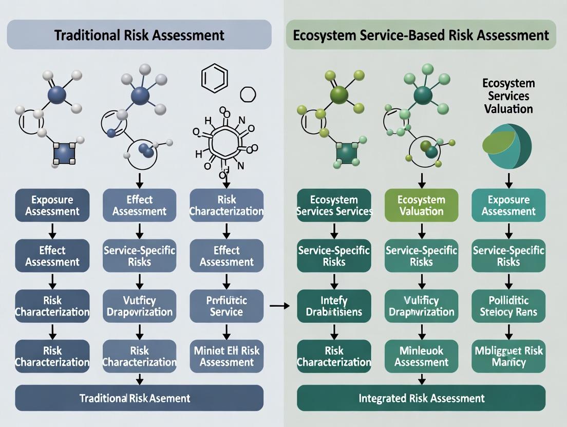
Core Principles and Historical Context: Deconstructing Traditional vs. Ecosystem Service Risk Assessment Paradigms

This guide compares two foundational paradigms in risk and impact assessment: the traditional chemical-centric Hazard Quotient (HQ) and the emerging human-centric Well-being Endpoint approach. The comparison is framed within a broader thesis contrasting traditional risk assessment with ecosystem service-based frameworks, which explicitly link ecological status to human welfare [1] [2].

The core distinction lies in their primary objective. The HQ paradigm is a protective, screening-level tool designed to identify if a single chemical exposure exceeds a toxicological threshold, thereby preventing harm [3] [4]. In contrast, the Well-being Endpoint paradigm is an integrative, evaluative tool aimed at quantifying the positive or negative impact of an intervention (e.g., a drug, environmental policy) on multidimensional human health and function [5] [6].

The following table summarizes their foundational differences:

Table 1: Foundational Comparison of Assessment Paradigms

Aspect	Hazard Quotient (HQ) Foundations	Human Well-being Endpoints
Primary Goal	To prevent adverse health effects from chemical exposure.	To quantify improvements in overall health, function, and quality of life.
Philosophical Basis	Reductionist, toxicological safety.	Holistic, geroscience/patient-centric benefit.
Typical Output	A dimensionless ratio (HQ). HQ < 1 indicates acceptable risk [3] [7].	Clinical outcomes (e.g., disability-free survival), composite indices, or validated biomarkers [5].
Regulatory Context	Central to EPA and ATSDR chemical risk assessments [3] [8].	Central to FDA clinical trial endpoints for drug approval [5] [6].
Ecosystem Service Link	Indirect; focuses on a chemical stressor's human health impact.	Direct; ecosystem services are explicitly valued for supporting human well-being (e.g., clean air, water, food) [1] [2].
Key Limitation	Can underestimate risk from aggregate or mixture exposure [9]; does not quantify benefit.	Can require large, long, and expensive trials to capture meaningful clinical events [5].

Foundational Principles and Calculation

Hazard Quotient (HQ) Methodology

The HQ is a deterministic, point-estimate ratio for screening-level risk. It is calculated by dividing an estimated exposure by a health-based guidance value [3] [7].

Core Equation: HQ = Exposure Dose (or Concentration) / Reference Value [3]

• Exposure Dose (D): Estimated daily intake (e.g., mg of chemical per kg body weight per day).
• Reference Value: A toxicological threshold such as:
  • Minimal Risk Level (MRL): Developed by ATSDR for acute, intermediate, and chronic exposures [3].
  • Reference Dose (RfD) or Reference Concentration (RfC): Developed by EPA for chronic oral and inhalation exposure, respectively [3] [8].

An HQ ≤ 1 suggests adverse non-cancer health effects are unlikely. An HQ > 1 indicates the exposure exceeds the reference value, warranting further investigation [3] [4]. For cumulative exposure to multiple chemicals affecting the same target organ, a Hazard Index (HI) is used, which is the sum of individual HQs [7] [4].

Example Calculation: For a chronic oral exposure to 1,2,3-trichloropropane at a dose of 0.50 mg/kg/day and an MRL of 0.005 mg/kg/day: HQ = 0.50 / 0.005 = 100. This high HQ indicates a significant exceedance of the health guideline [3].

Human Well-being Endpoint Methodology

Well-being endpoints are multidimensional constructs measured to reflect how a patient feels, functions, or survives [5]. Unlike the HQ's binary safety output, these endpoints measure a spectrum of benefit.

Selection of endpoints is critical and considers [5]:

• Link to Fundamental Biology: The endpoint should connect to the underlying biological process the intervention targets (e.g., cellular senescence, mitochondrial function).
• Salience: It must be meaningful to patients, clinicians, and regulators.
• Feasibility: It must be measurable within the practical constraints of a clinical trial.

The assessment relies on defined experimental protocols (see Section 4) to collect data on these endpoints, followed by statistical analysis to determine if a treatment effect is significant and clinically meaningful.

Pathway to a Validated Surrogate Endpoint: A major research focus is validating biomarkers (e.g., epigenetic age, SASP factors) as surrogate endpoints for long-term well-being. A valid surrogate must lie on the causal pathway between treatment and clinical outcome [5]. For example, treatment changes the biomarker, and the degree of biomarker change reliably predicts the magnitude of change in the final health outcome.

Diagram Title: The Deterministic Hazard Quotient (HQ) Risk Assessment Workflow

Diagram Title: The Integrative Pathway from Intervention to Human Well-being Endpoints

Comparative Analysis of Endpoints and Metrics

HQ-Based Metrics and Endpoints

HQ assessments rely on standardized toxicological endpoints derived from animal or epidemiological studies [8].

Table 2: Key Toxicological Endpoints for HQ Derivation

Endpoint Type	Definition	Role in HQ Paradigm
No-Observed-Adverse-Effect Level (NOAEL)	The highest tested dose where no adverse effects are observed.	Often used as the point of departure for deriving chronic RfDs/RfCs [8].
Lowest-Observed-Adverse-Effect Level (LOAEL)	The lowest tested dose where an adverse effect is observed.	Used if NOAEL is not identified; uncertainty factors are applied [8].
Benchmark Dose (BMD)	A statistical lower confidence limit on the dose producing a predefined low level of effect (e.g., 10%).	Increasingly preferred over NOAEL as it uses more of the dose-response data [8].
Critical Effect	The first adverse effect or its precursor that occurs as dose increases in the most sensitive species [8].	Determines the relevant endpoint and target organ for risk assessment.

Human Well-being Endpoints

Well-being endpoints are composite or direct measures of health status. Their validation for geroscience trials is an active area of research [5].

Table 3: Categories of Human Well-being Endpoints

Endpoint Category	Specific Examples	Advantages	Disadvantages/Challenges
Morbidity/Mortality	All-cause mortality; Disability-free survival.	High clinical relevance and face validity [5].	Rare events requiring large, long trials; mortality comprises diverse causes [5].
Disease-Specific	Incidence of Alzheimer's disease, cardiovascular events.	Clear regulatory path for drug approval [5].	May not capture simultaneous effects on multiple aging conditions [5].
Composite Indices	Advancing multimorbidity index; Frailty index; Deficit accumulation index.	Higher event rates increase statistical power; aligned with geroscience hypothesis [5].	No standardized tool; components may not be equally important or responsive [5].
Validated Surrogate Biomarkers	Hip bone mineral density (for fracture risk); Biological age estimators (under validation).	Can dramatically reduce trial size, duration, and cost [5].	Requires rigorous validation proving change in biomarker predicts change in clinical outcome [5].

Experimental Protocols and Data Generation

Protocol for HQ Determination

1. Problem Formulation & Hazard Identification: Review toxicological literature to identify the critical effect and relevant exposure routes (oral, inhalation, dermal) [8]. 2. Dose-Response Assessment: Identify the principal study and the point of departure (NOAEL, LOAEL, or BMDL). Apply uncertainty factors (UFs, typically multiples of 10) to account for interspecies extrapolation, intraspecies variability, database deficiencies, and LOAEL-to-NOAEL extrapolation [8]. The RfD is calculated as: RfD = NOAEL / (UF1 × UF2 × ...). 3. Exposure Assessment: Estimate the average daily dose (ADD) for the population: ADD = (C × IR × EF × ED) / (BW × AT), where C=contaminant concentration, IR=intake rate, EF=exposure frequency, ED=exposure duration, BW=body weight, AT=averaging time [4]. 4. Risk Characterization: Calculate the HQ. Perform uncertainty analysis describing the confidence in exposure and toxicity estimates [3].

Protocol for Establishing a Well-being Endpoint (e.g., in a Geroscience Trial)

1. Conceptual Alignment: Define the context of use and ensure the endpoint aligns with the biological mechanism targeted by the intervention [5]. 2. Endpoint Selection & Validation: * For novel digital endpoints: Follow the V3 framework: Verification (technical performance), Analytical Validation (accuracy against a gold standard), and Clinical Validation (association with a clinically meaningful outcome) [6]. * For composite clinical endpoints: Pre-specify all components and the rules for adjudicating an "event" [5]. 3. Trial Design: Determine if the endpoint is primary, secondary, or exploratory. For surrogate biomarkers, design studies to validate surrogacy—demonstrating that treatment-induced change in the biomarker predicts long-term clinical benefit [5]. 4. Data Collection & Analysis: Use standardized tools (e.g., validated questionnaires, performance tests, DHTs). Apply pre-specified statistical analysis plans to test the hypothesis of a treatment effect on the endpoint.

The Scientist's Toolkit: Essential Research Reagents and Materials

Table 4: Key Reagents and Tools for Risk and Benefit Assessment Research

Item / Solution	Primary Function	Relevant Paradigm
In Vitro Toxicity Assay Kits	High-throughput screening for cytotoxicity, genotoxicity, and specific organ toxicity (e.g., hepatotoxicity).	HQ Foundations: Early hazard identification.
Certified Reference Materials (CRMs)	Provide known, precise concentrations of chemicals for calibrating analytical instruments to ensure accurate exposure measurement (e.g., in food, water, soil).	HQ Foundations: Critical for reliable exposure assessment.
Animal Disease Models	Rodent or other animal models that simulate human diseases (e.g., Alzheimer's, atherosclerosis) or aging processes.	Both: Used for toxicological testing (HQ) and for proving mechanism/concept for well-being interventions.
Senescence-Associated Secretory Phenotype (SASP) Panel Assays	Multiplex immunoassays to quantify SASP factors (e.g., IL-6, MMPs) as biomarkers of cellular senescence.	Human Well-being: Target engagement and response biomarkers for senolytic therapies.
Epigenetic Clock Analysis Kits	Tools to measure DNA methylation patterns at specific CpG sites to estimate "biological age."	Human Well-being: A leading candidate biomarker for assessing gerotherapeutic interventions [5].
Validated Digital Health Technologies (DHTs)	Wearable sensors (actigraphy, ECG) or digital diaries to remotely and continuously collect real-world functional data (e.g., sleep, gait, heart rate).	Human Well-being: Enable collection of digitally derived endpoints in decentralized trials [6].
Ecosystem Service Models (e.g., InVEST)	Software models to map and quantify ecosystem services (e.g., water yield, carbon sequestration) and their supply-demand balance [2].	Bridging Tool: Links ecological data from traditional assessments to human well-being outcomes.

The field of risk assessment is undergoing a fundamental evolution, moving from models that examine isolated stressors to frameworks that embrace integrated system dynamics. Traditional paradigms, prevalent in toxicology and drug development, characterize risk through linear dose-response relationships and isolated hazard identification [10]. This approach often treats biological and ecological systems as closed entities. In contrast, a systems science perspective recognizes that a stressor perturbs a complex physiological or ecological system from its baseline state, potentially moving it into a new, lower-utility state within a different "attractor basin" [11] [12]. The cumulative cost of repeated responses to stressors is known as allostatic load, which represents a reduction in system utility and resilience [11].

Parallel to this thinking in human biology, environmental science has advanced the ecosystem services (ES) framework. This approach explicitly values the benefits that ecosystems provide to human well-being, such as provisioning, regulating, and cultural services [13]. Modern risk assessments now integrate these services as core components, recognizing that ecosystems are not just hazard sources but also provide critical mitigating functions (e.g., flood regulation, water purification) that reduce community vulnerability [1]. This evolution marks a shift from assessing isolated components to modeling the dynamic interactions within social-ecological systems, offering a more holistic basis for sustainable management and decision-making [13] [1] [14].

Comparison Guide: Traditional vs. Ecosystem Service-Based Risk Assessment

The following table provides a structured comparison of the foundational principles, methodologies, and outcomes of the traditional risk assessment paradigm versus the emerging ecosystem service-based framework.

Table 1: Comparison of Traditional and Ecosystem Service-Based Risk Assessment Approaches

Comparison Dimension	Traditional Risk Assessment (Isolated Stressors)	Ecosystem Service-Based Assessment (Integrated Dynamics)
Foundational Principle	Linear causality and threshold effects; focused on a single stressor or hazard [10].	System dynamics and complex interdependence; views stressors as perturbations to interconnected networks [11] [14].
Scope of Assessment	Narrow, focusing on direct toxicity, mechanism of action, and target organ effects [10].	Broad, encompassing social-ecological systems, including habitat quality, biodiversity, and human well-being [13] [1].
Key Outcome Metric	Allostatic Load: The cumulative physiological cost of adapting to repeated stressors, leading to reduced resilience [11].	Ecosystem Service Flow: The measurable capacity and actual use of benefits (e.g., water yield, soil stability) provided by ecosystems [13].
Vulnerability Consideration	Often limited to the sensitivity of a specific biological endpoint or population.	Explicitly integrates exposure, sensitivity, and adaptive capacity of both ecological and social subsystems [1].
Methodological Tools	Standardized toxicology studies, pharmacokinetic/pharmacodynamic (PK/PD) modeling [10].	Spatial modeling (e.g., InVEST), GIS mapping, and Structural Equation Modeling (SEM) to analyze direct/indirect social-ecological relationships [13].
Primary Application Domain	Drug development, chemical safety, occupational health [10] [15].	Environmental management, land-use planning, climate change adaptation, and natural hazard risk reduction [1].
Data Requirements	Controlled experimental data (in vitro, in vivo), clinical trial data [10].	Interdisciplinary data: ecological field data, remote sensing, socio-economic surveys, and Traditional Ecological Knowledge (TEK) [13].
Decision-Support Goal	Determine a "safe" dose or margin of safety for a specific agent [15].	Identify synergies and trade-offs between services to guide sustainable management and policy for resilient systems [13] [1].

Experimental Protocols for Integrated System Assessments

Implementing an ecosystem service-based risk assessment requires a multi-stage, integrative protocol. The following methodologies are adapted from contemporary environmental studies and framed for broader application [13] [1].

Protocol 1: Modular Social-Ecological Risk Assessment Framework This protocol is designed for regional-scale risk characterization, such as in coastal river deltas [1].

• Problem Formulation & Scoping: Define the spatial boundary (e.g., watershed, delta) and the suite of relevant ecosystem services (ES). For a drug development context, this could analogously involve defining the patient population, disease ecosystem, and relevant "services" like immune function or metabolic homeostasis.
• Indicator Library Development: Create a modular library of indicators for hazards, exposure, vulnerability, and ES capacity. For example, ES indicators may include quantifiable metrics for soil retention, water yield, or carbon sequestration [1].
• Spatial Data Integration: Collect and process geospatial data for all indicators using GIS. Perform multi-criteria analysis (e.g., Analytic Hierarchy Process) to weight and aggregate indicators into composite indices for hazard, vulnerability, and ES [1].
• Risk Visualization & Analysis: Generate composite risk maps by overlaying hazard, vulnerability, and ES layers. Identify areas of high risk and low ES provision. Statistically analyze drivers of risk profiles across different scales [1].

Protocol 2: Integrating Traditional Ecological Knowledge (TEK) with Quantitative ES Modeling This protocol focuses on incorporating qualitative social data into quantitative ecological models [13].

• Participatory ES Identification: Engage local communities or stakeholders through surveys, interviews, and participatory mapping to identify and prioritize culturally relevant ES (e.g., medicinal plants, aesthetic value) [13].
• Parallel Data Collection:
  • Ecological: Use field sampling and the InVEST model suite to quantify and map biophysical ES (e.g., habitat quality, nutrient retention) [13].
  • Social: Systematically document TEK related to resource use, ecological indicators, and management practices [13].
• Spatial Integration: Spatially overlay the TEK data layers with the biophysical ES and habitat quality maps in a GIS to identify areas of high socio-ecological value and potential conflict [13].
• Pathway Analysis: Use Structural Equation Modeling (SEM) to test and quantify the hypothesized direct and indirect relationships between social variables (e.g., TEK), ecological variables (e.g., habitat quality), and the final delivery of different ES categories [13].

System Dynamics and Workflow Visualization

Diagram 1: Causal Loop Diagram of Stress, Allostatic Load, and System Resilience [11] [12]

Diagram 2: Workflow for Integrated Ecosystem Service Risk Assessment [13] [1]

Table 2: Key Resources for Integrated System Dynamics Research

Tool/Resource	Primary Function	Application Context
InVEST Model Suite	A family of free, open-source software models used to map and value the goods and services from nature that sustain and fulfill human life [13].	Quantifying and spatially mapping ecosystem services like water yield, habitat quality, and carbon storage for scenario analysis.
Structural Equation Modeling (SEM)	A multivariate statistical analysis technique used to test complex networks of causal relationships between observed and latent variables [13].	Analyzing direct and indirect pathways linking social factors (e.g., traditional knowledge) and ecological factors to ecosystem service delivery.
Traditional Ecological Knowledge (TEK)	The cumulative body of knowledge, practice, and belief held by indigenous and local communities about their relationship with the environment [13].	Providing context-specific insights for ES identification, understanding ecological thresholds, and designing culturally appropriate management strategies.
Benefit and Risk Assessment & Management Plan (BRAMP)	A proposed lifecycle document to track the benefit-risk profile of a drug from development through post-marketing, enhancing decision transparency [15].	Implementing a dynamic, systems-oriented approach to drug safety that evolves with new evidence over time.
System Dynamics Software (e.g., Stella, Vensim)	Software for creating simulation models to understand the nonlinear behavior of complex systems over time using stocks, flows, and feedback loops [14].	Modeling complex interactions in social-ecological systems or pharmacological systems to simulate long-term outcomes under different scenarios.
GIS (Geographic Information Systems)	A framework for gathering, managing, and analyzing spatial and geographic data, essential for layering diverse information [13] [1].	Integrating spatial data on hazards, vulnerability, and ecosystem service provision to create composite risk maps.

The field of environmental risk assessment is undergoing a fundamental transformation, shifting from a traditional focus on isolated, single ecological endpoints to a comprehensive framework centered on ecosystem service bundles and their complex trade-offs and synergies [16] [17]. This paradigm change is driven by the need to connect ecological integrity directly to human well-being and to support more holistic environmental management and policy decisions [17]. Traditional risk assessment, often constrained to evaluating chemical stressors on specific organism-level receptors, is being augmented by approaches that quantify the supply and demand of multiple ecosystem services—such as water yield, carbon storage, and soil retention—and their spatial interactions [2] [18]. The integration of advanced modeling tools like InVEST and machine learning with concepts like ecosystem service vulnerability accounts enables researchers to predict risks under various scenarios and inform sustainable development strategies [19] [20]. This guide objectively compares these methodological frameworks, providing researchers and practitioners with the experimental data and protocols needed to implement next-generation, service-based risk assessments.

Methodological Comparison: Traditional vs. Ecosystem Service-Based Risk Assessment

The evolution from traditional ecological risk assessment (ERA) to ecosystem service (ES)-based frameworks represents a significant broadening of scope, objective, and analytical approach. The table below summarizes the core distinctions between these two paradigms.

Table 1: Comparative Framework: Traditional vs. Ecosystem Service-Based Risk Assessment

Aspect	Traditional Ecological Risk Assessment (ERA)	Ecosystem Service-Based Risk Assessment
Primary Objective	To estimate the likelihood of adverse effects on selected ecological receptors from a stressor (typically chemical) [17].	To evaluate risks to the continuous provision of ecosystem services that support human well-being and to analyze trade-offs among services [16] [17].
Focal Endpoints	Single or few assessment endpoints, often at the organism or population level (e.g., survival, reproduction of a test species) [17].	Bundles of final ecosystem services as endpoints (e.g., water provision, carbon sequestration, habitat quality) [16] [2].
Conceptual Basis	"Source-Stress-Exposure-Response" chain, focusing on a stressor's pathway and impact [2].	Ecosystem Production Functions and the supply-demand dynamic of services, linking ecological processes to human benefits [2] [17].
Spatial Consideration	Often local or site-specific, centered on the contamination or stressor source [17].	Explicitly spatial and regional, mapping service supply, demand, and mismatches (deficits/surpluses) across landscapes [2] [18].
Relationship Analysis	Not a central feature.	Central focus on quantifying trade-offs (increase in one service leads to decrease in another) and synergies (services increase or decrease together) [21] [18].
Valuation Dimension	Primarily ecotoxicological (e.g., LC50, NOEC). Limited economic valuation.	Integrates biophysical quantification with socio-economic valuation, explicitly connecting ecological change to human welfare [17].
Management Output	Aids in setting chemical safety standards or remediation goals for specific protection targets.	Informs landscape planning, natural resource management, and policy for optimizing multiple service flows and mitigating ES risks [16] [20].
Common Tools/Models	Laboratory bioassays, field surveys, probabilistic exposure models.	InVEST, ARIES, SoIVES models; GIS spatial analysis; machine learning for driver identification [20] [18].

The shift addresses a key limitation of traditional ERA: protecting a single species or lower-level endpoint does not necessarily ensure the protection of the broader suite of ecological functions that deliver benefits to people [17]. By making ecosystem services the explicit assessment endpoints, the framework ensures that management decisions aim for more comprehensive environmental protection [17].

Experimental Data & Performance Comparison

The performance of the ES-based approach is evidenced through its application in complex, real-world landscapes, revealing patterns invisible to traditional methods. The following experimental data from major studies highlights its analytical power.

Table 2: Comparative Experimental Data from Regional Ecosystem Service Assessments

Study Region & Focus	Key Ecosystem Services Assessed	Quantified Supply-Demand Dynamics (Sample Findings)	Identified Trade-offs/Synergies	Risk Bundle Classification
Xinjiang Uygur Autonomous Region (Arid Region) [2]	Water Yield (WY), Soil Retention (SR), Carbon Sequestration (CS), Food Production (FP)	WY Deficit: Demand (9.17×10¹⁰ m³) exceeded supply (6.17×10¹⁰ m³) in 2020, with deficit area expanding [2].CS Deficit: Rapid demand growth (4.38×10⁸ t) far outpaced supply (0.71×10⁸ t) [2].	Trade-off between water yield and other services in oasis expansion zones; synergies among regulating services in natural areas.	Four risk bundles identified (e.g., B1: WY-SR-CS high-risk; B4: Integrated low-risk), enabling targeted management [2].
Yunnan-Guizhou Plateau (Karst Region) [20]	Water Yield (WY), Carbon Storage (CS), Habitat Quality (HQ), Soil Conservation (SC)	Comprehensive ES index showed significant fluctuations (2000-2020), strongly linked to land-use change [20].	Complex web of trade-offs and synergies found; e.g., urban expansion created trade-off between provisioning services (food) and regulating services (CS, SC) [20].	Multi-scenario prediction (2035) showed the Ecological Priority scenario outperformed Natural Development and Planning-Oriented scenarios across all services [20].
Yellow River Basin [18]	Water Yield (WY), Carbon Storage (CS), Soil Conservation (SC), Habitat Quality (HQ), NPP	Clear spatial gradient: ES generally higher in upper reaches, lower in middle reaches [18].	WY had trade-off relationships with NPP, HQ, and CS. All other pairwise relationships were synergistic [18].	Three ES bundles identified: 1) WY & SC leading, 2) HQ & CS leading, 3) NPP leading [18].

The data consistently demonstrates that the ES-based framework successfully identifies spatially explicit mismatches between service supply and societal demand, which is a core component of modern ecological risk [2]. Furthermore, it quantitatively maps the complex interactions between services, showing that improving one (e.g., food production) often occurs at the expense of another (e.g., carbon storage or water quality), a critical insight for sustainable planning [21] [18].

Detailed Experimental Protocols

Implementing an ES-based risk assessment requires a structured, multi-stage workflow. The following protocols detail the standard methodologies derived from the cited research.

Table 3: Experimental Protocols for Ecosystem Service Bundle and Trade-off Analysis

Protocol Phase	Core Objectives	Standardized Methods & Models	Key Outputs
1. Biophysical Quantification	To spatially model and map the supply (capacity) of key ecosystem services.	- InVEST Model Suite: Uses land use/cover, climate, soil, and topographic data to quantify services like Water Yield, Sediment Retention, Carbon Storage, and Habitat Quality [2] [20] [18].- CASA Model: For quantifying Net Primary Productivity (NPP) [18].	Raster maps showing the spatial distribution and magnitude of each ecosystem service supply.
2. Supply-Demand Analysis	To identify areas of surplus, balance, and deficit for each service by comparing supply with demand.	- Spatial Overlay Analysis: Demand indicators (e.g., population density, agricultural land, water consumption) are spatially aligned with supply maps [2].- Supply-Demand Ratio (ESDR): Calculated as Supply / Demand to classify risk levels [2].	Maps of ES supply-demand ratios and risk classification (e.g., high deficit, low surplus).
3. Trade-off & Synergy Analysis	To statistically evaluate the relationships (positive/synergy, negative/trade-off) between pairs of services.	- Correlation Analysis: Pearson’s or Spearman’s rank correlation on service values across spatial units (e.g., pixels, watersheds) [18].- Spatial Correlation: Analyzes if spatial patterns of two services are significantly associated [18].- Production Possibility Frontiers: Visualize the feasible combinations of two services under different management scenarios [21].	Matrices of correlation coefficients and significance levels; graphs illustrating trade-off curves.
4. Risk Bundle Identification	To classify the landscape into homogeneous areas sharing similar ES supply-demand risk profiles.	- Self-Organizing Feature Map (SOFM): An unsupervised machine learning neural network for clustering multi-dimensional ES data [2] [18].- K-means Clustering: A simpler alternative for grouping areas based on normalized ES indices [20].	A zoning map of Ecosystem Service Risk Bundles (e.g., “High WY-SR Risk”, “Low Integrated Risk”).
5. Scenario Prediction & Driver Analysis	To forecast future ES changes under different socio-economic pathways and identify key influencing factors.	- PLUS Model: Simulates future land-use changes under designed scenarios (e.g., Natural Development, Ecological Priority) [20].- Machine Learning Regression: (e.g., Random Forest, Gradient Boosting) quantifies the relative importance of drivers (climate, land use, socio-economics) on ES patterns [20].	Future land-use and ES maps for 2030/2050; ranked lists of driver importance for each service.

Visualizing Conceptual and Analytical Frameworks

Diagram 1: Mechanistic Pathways for Ecosystem Service Relationships

This diagram illustrates the four pathways through which a driver of change (e.g., a policy or climate event) can lead to trade-offs or synergies between two ecosystem services (ES1 and ES2), as conceptualized by Bennett et al. (2009) [21].

Diagram 2: Integrated ES Risk Assessment Workflow

This diagram outlines the logical flow of a comprehensive ecosystem service-based risk assessment, from data preparation to management recommendations, integrating methodologies from the reviewed studies [2] [20] [18].

The Scientist's Toolkit: Essential Research Reagent Solutions

Table 4: Key Analytical Tools and Models for ES-Based Risk Assessment

Tool/Model Name	Category	Primary Function in ES Assessment	Application Example from Research
InVEST (Integrated Valuation of Ecosystem Services and Trade-offs)	Biophysical Modeling Suite	Spatially explicit models to quantify and map multiple ecosystem services (e.g., water yield, carbon storage, habitat quality) based on land use and biophysical data [20] [18].	Used as the core model for quantifying water yield, soil conservation, carbon storage, and habitat quality in studies across the Yellow River Basin, Yunnan-Guizhou Plateau, and Xinjiang [2] [20] [18].
PLUS (Patch-generating Land Use Simulation) Model	Land Use Change Model	Simulates future land-use changes under different scenarios by integrating demand forecasting and patch-level dynamics, providing essential input for future ES projections [20].	Applied to simulate land use in 2035 under Natural Development, Planning-Oriented, and Ecological Priority scenarios on the Yunnan-Guizhou Plateau [20].
Self-Organizing Feature Map (SOFM)	Machine Learning / Clustering	An unsupervised neural network algorithm used to identify and map ecosystem service bundles by clustering areas with similar ES supply, demand, or risk profiles [2] [18].	Used to classify the Xinjiang region into four distinct ecosystem service supply-demand risk bundles (B1-B4) for targeted management [2].
CASA (Carnegie-Ames-Stanford Approach) Model	Biophysical Model	Estimates terrestrial Net Primary Productivity (NPP)—a key indicator of ecosystem production and carbon sequestration service—using remote sensing and climate data [18].	Employed to evaluate the NPP service as part of the five-ES analysis in the Yellow River Basin [18].
Machine Learning Regression Models (e.g., Random Forest, Gradient Boosting)	Driver Analysis	Identifies and ranks the importance of various environmental and socio-economic drivers (e.g., precipitation, slope, GDP) influencing the spatial patterns of ecosystem services [20].	Used to determine that land use and vegetation cover were the primary factors affecting overall ecosystem services on the Yunnan-Guizhou Plateau [20].
Geographic Information System (GIS) Spatial Analyst	Spatial Analysis Platform	The foundational platform for managing, processing, and analyzing all spatial data layers, performing overlay analysis, calculating indices, and producing final risk maps [2] [18].	Integral to all cited studies for handling spatial data, conducting supply-demand overlay, and visualizing results [2] [20] [18].

The Driver-Pressure-State-Impact-Response (DPSIR) and Related Frameworks as Integrative Tools

This comparison guide evaluates the Driver-Pressure-State-Impact-Response (DPSIR) framework against its primary derivative and alternative models within the context of environmental risk assessment research. The analysis focuses on each framework's structure, methodological application, and suitability for integrating traditional risk paradigms with modern ecosystem service-based approaches. Quantitative evaluations and experimental case studies, including water governance and chemical risk assessment (e.g., PFAS), demonstrate that while DPSIR provides a robust foundational structure for causal chain analysis, evolved frameworks like DAPSI(W)R(M) and integrated models such as CSDA (Combined SWOT-DPSIR Analysis) offer superior capacity for handling socio-ecological complexity and quantifying impacts on human welfare. The findings indicate a clear trajectory from linear, pressure-centered models to iterative, service-oriented frameworks that are essential for sustainable policy implementation in drug development and environmental health [22] [23] [24].

The DPSIR framework, established by the European Environment Agency, is a causal model for organizing information about environmental problems [25]. It structures indicators into a chain of Drivers (socio-economic forces), Pressures (stressors on the environment), State (condition of the environment), Impacts (effects on ecosystem functions and human well-being), and societal Responses [26] [27]. Its primary strength lies in providing a common language for interdisciplinary communication between scientists, policymakers, and stakeholders [25].

However, criticisms of its terminological ambiguity, oversimplification of complex causal networks, and lack of explicit feedback loops have spurred the development of derivative frameworks [25] [23]. These derivatives aim to address specific shortcomings, such as better incorporating ecosystem services, human welfare, and governance structures.

The following table provides a core structural comparison of DPSIR and its major derivative frameworks.

Table 1: Core Structural Comparison of DPSIR and Derivative Frameworks

Framework	Core Components & Evolution	Primary Design Focus	Key Differentiator from DPSIR
DPSIR (Driver-Pressure-State-Impact-Response) [25] [27]	D → P → S → I → R	Structuring cause-effect chains for environmental reporting and policy communication.	The foundational linear model.
DPSWR (Driver-Pressure-State-Welfare-Response) [25] [23]	D → P → S → W → R	Explicitly linking environmental state changes to human welfare impacts.	Replaces "Impact" with "Welfare" to clarify the endpoint as human well-being.
DPSER (Driver-Pressure-State-Ecosystem Service-Response) [25] [28]	D → P → S → ES → R	Integrating Ecosystem Services (ES) as the critical link between state changes and human benefits.	Introduces ES as a formal component, bridging ecology and socio-economics.
DAPSI(W)R(M) [23] [28]	A(ctivities) → P → S → I(W) → R → M(easures)	Detailed accounting of human Activities, Welfare Impacts, and management Measures.	Elaborates Drivers into Activities, separates Welfare (W) from Impacts, and specifies Measures (M).
CSDA (Combined SWOT-DPSIR Analysis) [29]	SWOT (Strengths, Weaknesses, Opportunities, Threats) matrix integrated with DPSIR.	Strategic planning by combining internal/external contextual analysis (SWOT) with causal chains (DPSIR).	Adds a layer of strategic contextual and multi-criteria analysis to the DPSIR structure.

Performance Evaluation: Analytical Capabilities and Application

The practical utility of these frameworks is assessed through their analytical rigor, ability to integrate quantitative data, and effectiveness in guiding management responses. Performance is not uniform; it varies significantly with the complexity of the environmental system and the policy question at hand.

Table 2: Performance Evaluation of Frameworks in Key Analytical Dimensions

Analytical Dimension	DPSIR	DPSWR / DPSER	DAPSI(W)R(M)	CSDA (SWOT-DPSIR)
Causal Pathway Clarity	High for simple, linear chains. Low for complex, nested interactions [25] [23].	Moderate. Improved endpoint clarity (Welfare/Services), but retains linear simplification.	High. Detailed breakdown of Activities and Measures clarifies agency and management pathways [23].	Very High. SWOT contextualizes which DPSIR pathways are most strategically relevant [29].
Quantitative Integration Potential	Moderate. Often used with indicators, but links between components can be descriptive [24].	High for DPSWR (welfare metrics). Very High for DPSER (ecosystem service valuation).	High. Structure accommodates quantitative models linking Activities to Pressures and State changes [22].	Moderate. SWOT is qualitative; quantification depends on the DPSIR model it integrates with.
Handling Socio-Ecological Feedback	Poor. Lacks explicit feedback loops from Responses back to Drivers [25].	Poor. Retains essentially linear structure.	Good. The "Measures" (M) component is designed to feed back and alter "Activities" (A) [23] [28].	Good. SWOT analysis inherently considers feedback between internal/system and external/contextual factors.
Policy & Response Development	Good for identifying generic response types. Poor at prioritizing or evaluating effectiveness [25].	Good. Links responses directly to protecting Welfare or Ecosystem Services.	Excellent. Explicit "Measures" component forces consideration of concrete actions and their point of intervention [23].	Excellent. Prioritizes responses based on strategic fit (SWOT matrix).
Suitability for Ecosystem Service-Based Risk Assessment	Low. "Impact" is too broad and does not mandate ES consideration.	DPSER is specifically designed for this purpose.	High. The (W) component can be defined by changes in ecosystem service-derived welfare.	High. ES can be integrated as a key "Strength" or "Weakness" in the SWOT analysis.

Experimental Protocols and Case Study Applications

Protocol 1: Assessing Chemical Risks (PFAS) via Enhanced DPSIR

A 2023 study proposed a next-generation application of DPSIR for sustainable policy, using per- and polyfluoroalkyl substances (PFAS) as a case study [22]. The protocol enhances traditional DPSIR with five elements: iteration, risk/uncertainty analysis, flexible integration, quantitative methods, and clear definitions.

• Methodology:
  • Driver Definition: Identify industrial and consumer demand for water/stain-resistant products.
  • Pressure Quantification: Model emissions and environmental releases of PFAS throughout product life cycles.
  • State Monitoring: Measure PFAS concentrations in water, soil, biota, and human serum.
  • Impact Assessment: Quantify ecological toxicity and human health effects (e.g., carcinogenicity, immune effects) using epidemiological and toxicological data. Ecosystem service depletion (e.g., loss of drinking water security, fisheries) is explicitly calculated.
  • Response Simulation: Use quantitative models to test the effectiveness of potential responses (e.g., chemical bans, wastewater treatment upgrades) on reducing State and Impact metrics in an iterative feedback loop.
• Key Outcome: This approach demonstrated that moving beyond descriptive DPSIR to a quantitative, iterative model was critical for evaluating the cost-effectiveness and timeline of policy responses for complex contaminants [22].

Protocol 2: Water Governance Using DPSIR with Mass Balances

A 2018 study integrated DPSIR with water mass balance modeling to support evidence-based water governance [24]. This protocol addresses the criticism that DPSIR relations often remain descriptive.

• Methodology:
  • Construct a Conceptual DPSIR Model: For a river basin, define Drivers (e.g., agriculture), Pressures (e.g., nutrient runoff), State (e.g., nitrate concentration), Impact (e.g., eutrophication, cost of water treatment), and Responses (e.g., fertilizer regulations).
  • Develop a Quantitative Mass Balance Model: Create a hydrological and nutrient (e.g., nitrogen) balance model for the same basin.
  • Map DPSIR Components to Balance Model Parameters: Link "Pressure" to nutrient input terms, "State" to concentration in river compartments, and "Response" to manipulated input or removal rates in the model.
  • Scenario Analysis: Run the mass balance model under different "Response" scenarios to generate quantitative predictions for changes in "State" and "Impact" indicators.
• Key Outcome: The integration of a quantitative balance model transformed DPSIR from a communication tool into a predictive decision-support tool, allowing managers to compare the projected efficacy of different responses [24].

Protocol 3: Comparative Evaluation using Combined SWOT-DPSIR (CSDA)

A 2015 study formally compared DPSIR and the Combined SWOT-DPSIR Analysis (CSDA) approach using Multi-Criteria Decision Analysis (MCDA) [29].

• Methodology:
  • Independent Framework Application: Apply both standard DPSIR and CSDA to the same complex environmental management problem (e.g., desertification risk).
  • Criteria Generation: Define evaluation criteria such as "Ability to Handle Complexity," "Stakeholder Engagement Utility," and "Actionability of Outputs."
  • Expert Scoring: A panel of experts scores each framework's performance against the criteria.
  • MCDA Weighting and Ranking: Apply weights to the criteria based on project goals and compute a final performance score for each framework.
• Key Outcome: The study found CSDA consistently outperformed standard DPSIR in embracing system complexity and generating strategically prioritized responses, as it systematically accounts for internal and external contextual factors (via SWOT) that pure causal-chain analysis overlooks [29].

Core DPSIR Causal Chain: Illustrates the foundational linear sequence from Drivers to Responses.

Evolution from DPSIR to Derivative Frameworks: Maps the development of specialized frameworks from the core DPSIR model.

The Scientist's Toolkit: Essential Research Reagent Solutions

Table 3: Key Methodological "Reagents" for Framework Application

Tool/Reagent	Primary Function	Framework Application Context
Ecosystem Service Valuation Models (e.g., InVEST, ARIES)	Quantifies biophysical and economic value of ecosystem services (e.g., water purification, carbon sequestration).	Essential for populating the "Ecosystem Service" component in DPSER and for quantifying "Impacts" in service-based assessments using other frameworks [25] [28].
Mass Balance & Fate/Transport Models	Quantifies the movement and distribution of substances (water, nutrients, pollutants) through environmental compartments.	Critical for creating quantitative links between Pressures and State changes in DPSIR applications, as demonstrated in water governance studies [24].
Multi-Criteria Decision Analysis (MCDA) Software	Supports structured evaluation and ranking of decision options against multiple, often conflicting, criteria.	Used to formally compare frameworks (as in CSDA evaluation) or to prioritize "Responses" within any framework based on weighted social, economic, and ecological criteria [29].
Stakeholder Engagement Platforms (e.g., participatory mapping, deliberative workshops)	Facilitates the co-production of knowledge, identification of values, and validation of model assumptions.	Necessary for defining context-specific Drivers, Impacts, and acceptable Responses in all frameworks, moving beyond a purely technocratic analysis [22] [28].
Geographic Information Systems (GIS)	Visualizes and analyzes spatial data on Drivers, Pressures, State, and Impacts.	Used across all frameworks for spatially explicit analysis, identifying hotspots of pressure or impact, and planning targeted responses.
System Dynamics Modeling Tools	Simulates complex systems with feedback loops, delays, and non-linear interactions.	Addresses a key weakness of linear frameworks like DPSIR by modeling feedback from Responses to Drivers, suitable for advanced applications of DAPSI(W)R(M) [23].

Synthesis and Guidance for Research Application

The transition from traditional risk assessment (focused on isolated hazards and direct effects) to ecosystem service-based risk assessment (focused on system functions and human benefits) requires frameworks capable of integrating socio-ecological complexity. The analysis indicates:

• For foundational communication and linear problem structuring, the standard DPSIR framework remains a valid and widely understood starting point [26] [27].
• For research explicitly linking environmental change to human outcomes, DPSWR (welfare focus) or DPSER (ecosystem service focus) are superior choices, as they mandate the quantification of these endpoints [25] [23].
• For complex management scenarios requiring detailed intervention planning, DAPSI(W)R(M) provides the most granular structure for linking specific human activities to management measures [23] [28].
• For strategic policy development in contested or highly complex settings, CSDA (SWOT-DPSIR) offers the highest analytical power by integrating causal chain analysis with strategic contextual assessment [29].

The experimental data underscores that the integration of quantitative models (e.g., mass balances, ecosystem service valuation) within any chosen framework is critical to move from descriptive storytelling to predictive science that can robustly evaluate the potential outcomes of policy responses [22] [24]. For researchers and drug development professionals assessing environmental risks of pharmaceuticals or industrial chemicals, adopting an evolved framework like DPSER or DAPSI(W)R(M), coupled with stoichiometric and toxicological modeling, represents a state-of-the-art approach for demonstrating impacts on ecosystem services and human welfare.

From Theory to Practice: Methodological Frameworks and Applications in Research & Development

Ecological risk assessment (ERA) is the formalized process for evaluating the safety of manufactured chemicals and other anthropogenic stressors to the environment [30]. For decades, the cornerstone of this field has been a traditional toolkit built on controlled laboratory bioassays, the determination of lethal concentration (LC50) values, and tiered testing strategies designed to efficiently allocate resources [30] [31]. These methods prioritize standardization, reproducibility, and the establishment of clear cause-effect relationships for a limited set of model species under isolated conditions [30].

However, a fundamental challenge persists: a frequent mismatch between what is measured in the laboratory (e.g., individual organism survival) and the ultimate goal of protecting ecosystem-level attributes like biodiversity and function [30]. This gap has spurred the development of ecosystem service-based risk assessment frameworks. These approaches explicitly evaluate risks to the benefits humans derive from nature—such as clean water, pollination, or climate regulation—thereby directly linking ecological health to human well-being [32] [2]. This article provides a comparative guide, juxtaposing the established protocols and data outputs of the traditional toolkit with the emerging methodologies of ecosystem service-based analysis. It is framed within the broader thesis that while traditional methods provide essential, controlled toxicity data, integrating ecosystem service perspectives is critical for comprehensive environmental protection and sustainable management [30] [33].

The Traditional Toolkit: Core Methods and Protocols

The Foundation: Laboratory Bioassays and LC50 Determination

The laboratory bioassay is a fundamental technique where living organisms are used to detect or measure the biological activity of a substance, such as its toxicity. The LC50 (Lethal Concentration 50) is a specific, quantal endpoint from such assays, defined as the concentration of a chemical in air or water that is expected to cause death in 50% of a test population over a specified period, typically 24 to 96 hours [34].

• Experimental Protocol (Standard Aquatic LC50 Test):

  • Test Organism Selection: Standardized, sensitive species are used, such as the cladoceran Daphnia magna (water flea) or the fathead minnow (Pimephales promelas) [30].
  • Exposure System: Groups of organisms are placed in a series of test chambers (e.g., beakers, flow-through cells) containing the chemical at different concentrations, plus a control group with no chemical.
  • Duration & Conditions: The test runs for a fixed period (e.g., 48 or 96 hours) under controlled temperature, light, and water quality conditions (pH, dissolved oxygen) [34].
  • Endpoint Measurement: Mortality (the quantal effect) is recorded at regular intervals. The LC50 value and its confidence limits are then calculated using statistical methods like probit or logistic regression analysis [34].

• Key Performance Data: LC50 values allow for the comparative ranking of chemical acute toxicity. A lower LC50 indicates higher toxicity. For example, dichlorvos, an insecticide, has an inhalation LC50 (rat, 4-hour) of 1.7 ppm, classifying it as "extremely toxic" via that route, while its oral LD50 (rat) of 56 mg/kg classifies it as "moderately toxic" [34].

Tiered Testing Strategy: A Risk-Based Screening Framework

Tiered testing is a resource-efficient strategy designed to handle large numbers of chemicals [31]. It operates on a "screen-first" principle, where simple, low-cost assays are used to prioritize substances for more complex and costly testing [30] [31].

• Theoretical Basis: The strategy combines chemical, toxicological, and decision-theoretical knowledge. It aims to maximize the utility (e.g., protection of health, cost-saving) of testing by minimizing false negatives (missing a hazardous chemical) and false positives (unnecessarily regulating a safe one) within resource constraints [31].
• Standard Four-Tier Workflow: The process is iterative, with each tier providing a more refined risk estimate [30].

Diagram: Traditional Tiered Ecological Risk Assessment Workflow [30].

• Comparative Data Across Tiers: The following table summarizes the progression in complexity, cost, and output from Tier I to Tier IV.

Table 1: Characterization of a Four-Tiered Ecological Risk Assessment Framework [30].

Tier	Description	Primary Risk Metric	Example Methods	Cost & Complexity
Tier I	Conservative screening to "screen out" chemicals with no conceivable risk. Uses worst-case exposure and single-species toxicity values.	Hazard Quotient (HQ = Exposure/Effect). Compared to a Level of Concern (e.g., HQ > 1 indicates potential risk).	Deterministic comparison of estimated environmental concentration (EEC) to LC50/EC50.	Low cost, high throughput, highly conservative.
Tier II	Refined analysis incorporating variability and uncertainty in exposure and effects.	Probabilistic estimate of the likelihood of an adverse effect.	Species Sensitivity Distributions (SSDs) to derive a Protective Concentration (e.g., HC₅).	Moderate cost, begins to quantify uncertainty.
Tier III	Complex modeling with biologically and spatially explicit scenarios. Explores interaction of stressors and recovery.	Probabilistic population- or community-level risk estimates.	Mechanistic effect models, population models, refined exposure modeling.	High cost, data intensive, reduced conservatism.
Tier IV	Site-specific, environmentally relevant data collection under real-world conditions.	Multiple lines of evidence from field studies.	Mesocosm or field studies, ecosystem monitoring, biomarker studies.	Very high cost, most environmentally realistic.

The Ecosystem Service-Based Approach: Frameworks and Metrics

In contrast to the toxicological focus of traditional ERA, the ecosystem service (ES) approach evaluates risk by analyzing threats to the supply and demand of nature's benefits [2]. The core thesis is that risk is not merely a function of toxicity and exposure, but of the imbalance between human demand for services and the ecosystem's capacity to supply them [2] [33].

Core Conceptual Shift: From Receptor to Service

The assessment endpoint shifts from protecting a test species (measurement endpoint) to protecting a specific service flow, such as water yield for drinking or carbon sequestration for climate regulation [2]. A key framework for structuring this analysis is the Driver–Activities–Pressures–State–Impact (Welfare)–Response (DAPSI(W)R) model, which links human activities to changes in ecosystem state and ultimately to impacts on human welfare [33].

Experimental & Analytical Protocols

ES-based risk assessment often relies on spatial modeling, expert elicitation, and trend analysis, rather than standardized laboratory bioassays.

• Protocol for Spatial Supply-Demand Risk Assessment (as used in Xinjiang study [2]):

  • Service Selection: Identify key ES relevant to the region (e.g., water yield (WY), soil retention (SR), carbon sequestration (CS), food production (FP)).
  • Quantification of Supply: Use biophysical models (e.g., InVEST model suite) with spatial data (land use, soil, climate) to map the capacity of ecosystems to provide each service.
  • Quantification of Demand: Map human demand for each service using socio-economic data (population, irrigation needs, carbon emissions, food consumption).
  • Risk Identification: Calculate a Supply-Demand Ratio (SDR). An SDR < 1 indicates a deficit (supply < demand), representing ecological risk. Incorporate trend indices (Supply Trend Index, Demand Trend Index) to assess whether deficits are growing or shrinking [2].
  • Risk Bundling: Use clustering algorithms (e.g., Self-Organizing Feature Maps) to identify areas with similar ES risk profiles, guiding targeted management [2].

• Protocol for Expert-Based Risk Assessment (as used in the Barents Sea study [33]):

  • Structured Elicitation: Engage experts familiar with the socio-ecological system.
  • Framework Application: Use the DAPSI(W)R framework to list human Activities (e.g., fishing, shipping) and resulting Pressures (e.g., bycatch, pollution). Use the CICES framework to classify affected Ecosystem Services.
  • Risk & Certainty Scoring: Experts score the risk (combination of likelihood and impact) of each Activity-Pressure combination on each ES. They also score their own certainty in each assessment.
  • Analysis: Aggregate scores to identify high-risk, high-certainty priorities for immediate management and high-risk, low-certainty topics for urgent research [33].

Diagram: Core Workflows for Ecosystem Service-Based Risk Identification [2] [33].

• Comparative ES Risk Data: The Xinjiang study (2000-2020) provides quantitative, spatially explicit risk data based on SDR [2]. The Barents Sea study provides qualitative risk rankings derived from expert judgment [33].

Table 2: Comparative Outputs from Ecosystem Service-Based Risk Assessments.

Study & Approach	Ecosystem Services Analyzed	Key Risk Metrics	Example Finding
Xinjiang (Spatial Modeling) [2]	Water Yield (WY), Soil Retention (SR), Carbon Sequestration (CS), Food Production (FP)	Supply-Demand Ratio (SDR), Trend Indices.	From 2000 to 2020, the CS demand grew nearly 8x (0.56×10⁸ t to 4.38×10⁸ t) while supply increased only 1.6x, indicating a sharply growing deficit and high risk.
Barents Sea (Expert Elicitation) [33]	Fish/Shellfish (Provisioning), Biodiversity (Cultural), Education, etc.	Expert-ranked risk (Low-Medium-High) and certainty score.	Fish/Shellfish provision and Biodiversity were identified as the two most threatened ES, with temperature change being the most impactful pressure.

Integrated Comparison and Future Directions

The traditional and ES-based approaches offer complementary strengths and weaknesses, which are compared in the table below. The future of robust ERA lies in strategic integration.

Table 3: Comparison of Traditional Toxicological and Ecosystem Service-Based Risk Assessment Approaches.

Aspect	Traditional Toolkit (Bioassays & Tiered Testing)	Ecosystem Service-Based Approach
Primary Endpoint	Survival, growth, reproduction of individual model organisms.	Maintenance of service flows (supply vs. demand) to human society.
Core Metric	Toxicity values (LC50, NOEC), Hazard Quotient (HQ).	Supply-Demand Ratio (SDR), risk to service provision.
Strengths	High cause-effect clarity; standardized, reproducible; excellent for chemical ranking and early screening; quantitative dose-response [30] [31].	Directly links ecology to human welfare; identifies spatially explicit management zones; accounts for multiple, cumulative stressors; holistic system perspective [32] [2] [33].
Limitations	High uncertainty in extrapolation from lab to field, from few species to ecosystems; often ignores ecological interactions and recovery; mismatch with protection goals [30].	Can be data and resource intensive; complex models with high uncertainty; lack of standardized protocols; challenging to establish direct causality for specific chemicals [33].
Optimal Application	Mandatory regulatory screening of new chemicals; establishing baseline toxicity; cause-investigation of point-source pollution.	Landscape-level planning and management; assessing impacts of climate change, land-use change, and multiple stressors; communicating risk to stakeholders [2] [33].

The Path Forward: Hybrid and Next-Generation Frameworks

The trajectory of ERA is moving toward evidence-based integration, where data from traditional bioassays, in vitro systems, "-omics," and ES models are combined within structured, weight-of-evidence frameworks [35]. Promising developments include:

• Bioassay-Machine Learning Integration: Enhancing traditional bioassays by using machine learning models (e.g., gradient boosting) on bioassay data to improve toxicity prediction and scalability [36].
• Network Theory Applications: Using complex network analysis to model interactions within socio-ecological systems, improving understanding of ES cascades and trade-offs [37].
• Adverse Outcome Pathways (AOPs) Linked to ES: Connecting molecular initiating events from traditional toxicology to organism- and population-level outcomes that ultimately affect ecosystem service provision [30].

The Scientist's Toolkit: Essential Research Reagents and Materials

Table 4: Key Research Reagent Solutions and Materials for Featured Methods.

Item	Function/Description	Primary Application
Standard Test Organisms (e.g., Daphnia magna, Ulva australis, Fathead minnow)	Sensitive, well-characterized biological models for quantifying toxicological effects in controlled experiments.	Laboratory Bioassays [30] [36] [34].
Reference Toxicants (e.g., Potassium dichromate, Sodium dodecyl sulfate)	Standard chemicals with known and reproducible toxicity used to validate the health and sensitivity of test organism cultures.	Quality assurance/control for bioassays.
Herbicides/Analytes for Bioassay (e.g., Diuron, Atrazine, Hexazinone)	Pure-form chemical stressors used to establish dose-response curves and calculate EC50/LC50 values.	Toxicity testing and chemical ranking [36] [34].
Artificial Seawater/Test Media	Chemically defined water that replicates natural conditions (salinity, pH, hardness) to ensure test reproducibility.	Aquatic bioassays with marine/estuarine species [36].
InVEST Model Suite Software	A family of open-source, GIS-based software models for mapping and valuing ecosystem services.	Quantifying and spatially analyzing ES supply [2].
CICES and DAPSI(W)R Framework Guides	Classification systems and conceptual models that provide standardized terminology and structure for ES identification and risk analysis.	Designing and conducting ES-based risk assessments [33].
Expert Elicitation Protocols	Structured questionnaires, workshop formats, and scoring sheets designed to systematically gather and synthesize expert judgment.	Qualitative and semi-quantitative ES risk assessment where empirical data is lacking [33].

The quantification of ecosystem service (ES) supply, demand, and their spatial mismatch represents a pivotal methodological advancement in environmental science. This evolution marks a significant shift from traditional risk assessment paradigms, which predominantly focused on chemical stressors and their impacts on selected organism-level receptors or on landscape pattern analysis [17] [2]. Traditional ecological risk assessment (ERA) often operated with the implicit assumption that protecting foundational biological levels would consequently safeguard higher ecosystem functions and human well-being, a linkage that was frequently untested [17].

In contrast, ecosystem service-based risk assessment explicitly centers on the benefits that ecosystems provide to people, framing environmental protection in terms of sustaining final services like clean water, food, climate regulation, and cultural benefits [17]. This approach directly connects ecological integrity to human health and societal welfare, thereby providing a more comprehensive and societally relevant framework for environmental management and decision-making [1]. By quantifying ES supply (the capacity of an ecosystem to provide a service) and demand (the human consumption or requirement for that service), researchers can identify deficits, pressure points, and mismatches that constitute novel forms of ecological risk [38] [2]. Integrating this supply-demand dynamic into risk assessments broadens the range of potential management and risk reduction measures, allowing policymakers to consider strategies that enhance natural capital alongside conventional engineering or regulatory solutions [1]. The following conceptual diagram illustrates this paradigm shift from a traditional stressor-receptor model to an integrated ecosystem service supply-demand risk framework.

Comparative Guide to Primary Quantification Methodologies

A wide array of methodologies has been developed to quantify ES supply and demand, ranging from simple empirical equations to complex process-based models. A systematic review of 862 publications identified 47 distinct methods, 1,130 equations, and 1,190 parameters used in urban ES studies alone, indicating a vibrant and diverse methodological field [39]. The choice of method involves critical trade-offs between complexity, data requirements, spatial explicitness, and the intended use of the results for management or policy.

Table 1: Comparison of Primary Ecosystem Service Quantification Methodologies

Methodology Category	Typical Spatial Resolution	Temporal Dynamics	Key Strengths	Primary Limitations	Common Applications in Risk Assessment
Look-up Tables & Value Transfer	Coarse (Regional/National)	Static (single time point)	Low data & expertise requirement; rapid assessment.	High uncertainty; ignores local context & spatial heterogeneity.	Preliminary screening; national-scale assessments [39].
Empirical Equations & Simple Indices	Medium to Fine (Landscape/City)	Can be multi-temporal	Moderately complex; balances accuracy & feasibility.	Relies on generalized parameters; process representation limited.	Urban ES bundles; landscape pattern-risk analysis [39] [40].
Biophysical Process Models (e.g., InVEST, SWAT)	Fine (Watershed/Grid)	Dynamic (can project trends)	Spatially explicit; models ecological mechanisms.	High data input & calibration needs; computationally intensive.	Watershed management; climate change impact studies [2] [41].
Integrated Socio-Ecological Frameworks	Multi-scale (Nested)	Dynamic	Captures human demand & social drivers explicitly.	Requires interdisciplinary data; complex integration.	Social-ecological risk; policy scenario evaluation [38] [1].

The InVEST (Integrated Valuation of Ecosystem Services and Tradeoffs) model suite, developed by the Natural Capital Project, is a prominent example of a spatially explicit, process-based modeling approach. It enables the mapping and valuation of multiple ES (e.g., water yield, carbon sequestration, habitat quality) under different land-use scenarios. For instance, in a risk assessment of Xinjiang, the InVEST model was used to quantify the supply of four key services—water yield, soil retention, carbon sequestration, and food production—from 2000 to 2020 [2]. This biophysical supply was then compared to spatially explicit demand metrics, calculated based on population, economic density, and land use, to identify high-risk deficit areas [2].

A critical insight from comparative reviews is that simpler methods are used more frequently than complex ones, likely due to constraints related to data, transparency, and technical capacity [39]. Notably, a significant transparency gap exists: more than 60% of reviewed studies did not fully specify the sources or values of the parameters used in their equations, hindering reproducibility and robust risk analysis [39].

Core Experimental Protocols for Quantifying Supply-Demand Mismatch

A robust experimental protocol for ES mismatch analysis involves sequential steps of quantification, comparison, and risk characterization. The following workflow, synthesized from multiple recent studies, provides a generalizable template.

General Experimental Workflow:

• Definition of Study System and Scales: Define the geographical boundary (e.g., watershed, urban area, region) and critically select the administrative and/or grid-based analytical scales. Multi-scale analysis (e.g., county and 3km grid) is recommended as supply-demand relationships and their drivers can vary significantly with scale [38].
• Selection and Quantification of Ecosystem Services: Select final ES relevant to the study area's risk profile. Use biophysical models (e.g., InVEST for water yield, carbon storage), remote sensing data (for NPP, vegetation cover), or validated empirical equations to map the biophysical supply of each service across the landscape [2] [41].
• Spatialization of Societal Demand: Quantify and map the demand for each ES. Demand proxies vary by service: e.g., population density and water use for water provision; population and GDP density for climate regulation and recreation; livestock numbers for forage [40] [42]. Demand is often normalized and mapped to a comparable spatial unit (e.g., per grid cell).
• Calculation of Mismatch Indices: Calculate a spatialized index comparing supply and demand. Common metrics include:
  • Ecosystem Service Supply-Demand Ratio (ESDR): ESDR = (Supply - Demand) / Supply, or a simple Supply/Demand ratio [2]. Values < 0 indicate a deficit (demand > supply).
  • Local Gini Coefficient: An inequality measure adapted with spatial moving windows to quantify the inequality in ES supply and demand distribution within a local neighborhood, addressing spatial autocorrelation [40].
• Risk Identification and Bundling: Classify areas into risk categories (e.g., high deficit, balance, surplus) based on mismatch indices. Advanced studies use clustering algorithms like Self-Organizing Feature Maps (SOFM) to identify "risk bundles"—areas with similar combinations of deficits across multiple ES. This reveals integrated, multi-service risk profiles crucial for management [2].
• Analysis of Drivers and Future Scenarios: Use statistical models (e.g., Principal Component Analysis, Bayesian Networks) to identify key social-ecological drivers (e.g., land-use change, population, climate variables) of the observed mismatches [38] [42]. Model future scenarios (e.g., urban expansion, climate change) to project evolving risks.

Table 2: Exemplar Experimental Data from Recent Supply-Demand Mismatch Studies

Study Region	Key Ecosystem Services Analyzed	Quantified Supply-Demand Trend (2000-2020)	Primary Identified Risk Driver	Reference
Xinjiang, China (Arid Region)	Water Yield (WY), Soil Retention (SR), Carbon Sequestration (CS), Food Production (FP)	WY demand grew faster than supply; CS deficit expanded sharply (demand: 0.56→4.38 x10⁸ t); FP surplus increased.	Water scarcity; rapid urbanization and associated carbon emissions.	[2]
Iran (Arid/Semi-Arid)	Forage, Water Yield, Medicinal Plants, Mushroom, Carbon, Pollination, Recreation, Aesthetic	>60% of country deficient in ≥1 service. Largest deficits: Forage (78% of area), Pollination (75%).	Population pressure & land-use change (Bayesian Network identification).	[42]
Danjiangkou Basin, China	Composite based on land use, population, and economic density.	Inequality in supply-demand intensified over time, showing strong spatial heterogeneity.	Urbanization level; spatial compactness of development mitigated inequality.	[40]
Northern Tianshan Mountains, China	Food Provision, Water Retention, Soil Conservation, Carbon Sequestration, Habitat Quality.	Worsening overall imbalance. Trade-offs (e.g., between food provision and other services) were scale-dependent.	Natural factors dominant at fine scale; anthropogenic factors more prominent at county scale.	[38]

The following diagram details the standard analytical workflow for implementing this protocol, from data preparation through to risk visualization and management feedback.

The Scientist's Toolkit: Essential Research Reagent Solutions

Conducting robust ES supply-demand analysis requires a suite of key tools, datasets, and models. The following toolkit is compiled from the infrastructure commonly employed and cited in the current literature.

Table 3: Essential Research Toolkit for ES Supply-Demand and Mismatch Analysis

Tool/Reagent Category	Specific Examples	Function in Analysis	Key Considerations & Sources
Geospatial Data Platforms	Google Earth Engine; USGS Earth Explorer; ESA Copernicus Open Access Hub.	Provides access to remote sensing imagery (Landsat, Sentinel) and global datasets for land cover, climate, and topography.	Enables large-scale, reproducible analyses. Critical for calculating vegetation indices and land-use change [41].
Biophysical ES Modeling Software	InVEST (Integrated Valuation of Ecosystem Services and Tradeoffs); Soil and Water Assessment Tool (SWAT).	Simulates the biophysical production of services (water yield, sediment retention, carbon storage, habitat quality) based on input maps.	The InVEST model is explicitly designed for ES mapping and scenario analysis. Requires careful parameterization and calibration [2].
High-Resolution ES Datasets	China 30m ES Dataset (2000-2020) [41]; Global datasets from NASA SEDAC.	Provides pre-processed, validated maps of ES supply (NPP, water yield, soil conservation) for validation or direct use.	Reduces computational burden. Ensures consistency for national/regional comparisons. Must assess uncertainty [41].
Statistical & Clustering Software	R (with spdep, ggplot2, cluster packages); Python (SciPy, scikit-learn); ArcGIS; QGIS.	Performs spatial statistics (Local Gini, Moran's I), driver analysis (PCA, regression), and risk bundling (SOFM, K-means).	Essential for moving from mapped quantities to analysis of inequality, drivers, and risk classification [40] [2].
Social-Economic Demand Data	National census data; WorldPop gridded population; Global GDP grids; National land use/cover maps.	Provides the spatialized proxies for ES demand (population density, economic activity, land development intensity).	Crucial for representing the "demand" side. Downscaling and reconciling data formats is a major methodological step [40] [42].

The methodology for quantifying ES supply, demand, and mismatch has matured into a sophisticated toolkit that fundamentally reframes ecological risk. By moving beyond the traditional focus on stressors and organismal receptors, this approach directly links ecosystem integrity to human well-being, identifying risk as a function of the gap between what nature provides and what society requires [17] [1]. Key methodological advances include the move toward multi-scale and spatially explicit analyses, the development of composite indices for inequality (e.g., local Gini coefficient), and the use of clustering techniques to identify integrated risk bundles [38] [40] [2].

The evidence strongly supports the integration of ES into formal risk assessment. Studies demonstrate that incorporating ES provides a more comprehensive view of vulnerability, particularly in complex social-ecological systems like coastal deltas or arid regions [1] [42] [2]. It reveals that drivers of risk are scale-dependent (with anthropogenic factors like urbanization becoming more prominent at broader administrative scales) [38] and that synergies and trade-offs between services are central to understanding risk dynamics [42]. Future methodology development must prioritize: 1) enhancing the transparency and reproducibility of parameter sources in models [39]; 2) better integration of dynamic social demand models with biophysical supply models; and 3) strengthening the linkage between quantified mismatch indices and concrete, hierarchical governance actions for risk reduction [40] [1]. As these methodologies continue to standardize and improve, they offer a powerful, evidence-based pathway for aligning environmental management with the dual goals of ecosystem sustainability and human welfare.

Conceptual Foundation: Traditional vs. Ecosystem Service-Based Risk Assessment

Ecological risk assessment (ERA) has evolved through distinct paradigms, fundamentally shaping how landscapes are analyzed and risks are mapped. The traditional paradigm, rooted in toxicology and conservation biology, focuses on discrete stressors and their impacts on specific ecological receptors or indicator species [43]. This reductionist approach quantifies risk through metrics like the probability of fatality for selected species or landscape pattern indices, often prioritizing scientific precision and reliability over comprehensiveness [43] [44] [30]. Its spatial applications frequently involve analyzing land use/land cover (LULC) change to calculate landscape disturbance and vulnerability indices [2] [44].

In contrast, the ecosystem service-based paradigm adopts a wholistic framework centered on human well-being [43] [45]. It defines risk through the lens of ecosystem service (ES) degradation, measuring the mismatch between the supply of services (e.g., water yield, carbon sequestration) and societal demand [2]. This approach explicitly links ecological processes to human welfare, making it inherently interdisciplinary and stakeholder-relevant [43] [46]. The spatial-explicit analysis in this paradigm maps the flows, synergies, and trade-offs of multiple ES across landscapes [47].

The core distinction lies in the assessment endpoint: traditional ERA aims to protect ecological structures and indicator species, while ES-based ERA (ESRA) aims to safeguard the functions and services that ecosystems provide to people [45] [30]. This shift reframes the landscape from a mosaic of habitats and stressors to a dynamic, multi-functional provider of benefits, necessitating more complex spatial models that incorporate both biophysical and socio-economic data flows [2] [47].

Comparative Framework of Methodological Approaches

The following table summarizes the core differences between the two paradigms across key dimensions of spatial-explicit analysis.

Table 1: Comparison of Traditional and Ecosystem Service-Based Risk Assessment Paradigms

Dimension	Traditional Landscape ERA	Ecosystem Service-Based ERA (ESRA)
Primary Assessment Endpoint	Health of indicator species, ecological structures (e.g., habitat patches), absence of contamination [43] [30].	Sustained provision of ecosystem services (ES) to human beneficiaries (e.g., clean water, flood regulation) [2] [45].
Core Risk Metric	Probability of adverse effect on receptor; Landscape indices (disturbance, fragmentation, vulnerability) [44] [30].	Supply-demand mismatch ratio for ES; Risk of ES deficit or functional connectivity loss [2] [47].
Spatial Modeling Focus	Habitat suitability, landscape connectivity for target species, LULC change simulation [48] [44].	Mapping ES supply areas, demand zones, flow paths, and functional connectivity between service-providing units [2] [47].
Scale Considerations	Often species-specific or landscape-pattern driven; Can struggle with cross-scale integration [30].	Explicitly multi-scale, linking local ES production to regional demand and management jurisdictions [46] [47].
Key Data Inputs	Species occurrence data, LULC maps, toxicological data [48] [44].	Biophysical models (e.g., InVEST), socio-economic demand data, stakeholder valuations [46] [2].
Strength	Scientifically precise, standardized, strong causal inference for specific stressors [43] [30].	Policy-relevant, connects ecology to human well-being, captures ecosystem complexity and multifunctionality [46] [45].
Weakness	May miss ecosystem-wide effects and human benefits; Can be narrow in scope [43] [30].	Data intensive, complex modeling with uncertainties; Challenges in validating service flows [46] [45].

Experimental Protocols for Spatial-Explicit Analysis

Protocol 1: High-Resolution Habitat and Connectivity Modeling (Traditional Paradigm)

This protocol, derived from a bat conservation study, exemplifies the traditional paradigm's application in spatial planning [48].

• Species-Centric Data Collection: Fit target species (e.g., greater horseshoe bat, Rhinolophus ferrumequinum) with GPS telemetry loggers to gather fine-scale movement and habitat use data over relevant seasons [48].
• High-Resolution Landscape Mapping:
  • Generate a land classification map using satellite imagery (e.g., Sentinel-2).
  • Create a detailed vegetation structure map using airborne Light Detection and Ranging (LiDAR) data to capture canopy height and density [48].
• Model Development & Validation:
  • Habitat Suitability Modeling: Use telemetry data as presence points in a model (e.g., MaxEnt, Resource Selection Function) with environmental layers (land cover, vegetation structure, distance to water) as predictors.
  • Landscape Connectivity Modeling: Apply circuit theory or least-cost path analysis using the habitat suitability map as a resistance surface.
  • Validate model predictions using an independent dataset (e.g., field surveys or acoustic monitoring data not used in model training) [48].
• Risk Mapping & Planning Integration: Overlay high-resolution connectivity and suitability maps with proposed development zones. Identify and prioritize critical corridors and core habitats for avoidance or mitigation [48].

Protocol 2: Ecosystem Service Supply-Demand Risk Mapping (ESRA Paradigm)

This protocol, based on a study in Xinjiang, China, details an ESRA approach for arid regions [2].

• ES Selection and Quantification:
  • Select key ES relevant to the region (e.g., Water Yield (WY), Soil Retention (SR), Carbon Sequestration (CS), Food Production (FP)).
  • Supply Quantification: Use biophysical models (e.g., the InVEST suite) with input data including LULC maps, soil data, precipitation, and DEM to map the spatial supply of each ES for multiple time points [2].
• Demand Quantification & Spatial Allocation:
  • Define demand indicators (e.g., water consumption for WY, population distribution for FP).
  • Spatially allocate demand using statistical data at municipal/county levels, often distributing it based on population density or land use type [2].
• Supply-Demand Risk Calculation:
  • Calculate a Supply-Demand Ratio (SDR) for each ES at the pixel or administrative unit level: SDR = Supply / Demand.
  • Calculate Trend Indices (Supply Trend Index - STI, Demand Trend Index - DTI) to analyze changes over time.
  • Classify risk levels (e.g., deficit, balanced, surplus) based on SDR thresholds and trends [2].
• Spatial Risk Bundling and Zoning:
  • Use a clustering algorithm (e.g., Self-Organizing Feature Map - SOFM) on the multi-ES risk layers to identify ES risk bundles—areas sharing similar multi-ES risk profiles.
  • Map these bundles to guide differentiated management policies (e.g., B1: WY-SR-CS high-risk area requires strict conservation) [2].

Protocol 3: Mapping Functional Connectivity of Multiple Ecosystem Services

This advanced ESRA protocol focuses on modeling the spatial interdependencies between ES [47].

• Foundation ES Supply Mapping: Map the supply areas for multiple ES (e.g., plant agriculture, water flow regulation, aesthetics) using standard models (e.g., InVEST) or proxy indicators [47].
• Theoretical Linkage Definition: For each pair of ES, define the directional ecological process linking them (e.g., water flow from regulation areas supports irrigation for agriculture downstream). Represent these as network edges with a weight (strength of interaction) [47].
• Spatial Connectivity Modeling:
  • Conceptualize the landscape as a network. ES supply areas are nodes.
  • For abiotic flows (e.g., water), use hydrological routing models. For biotic flows (e.g., pollination), use least-cost path or circuit theory based on habitat resistance.
  • Model the "functional connectivity" of ES by mapping the predicted flow paths of the mediating process (water, species movement) between source and beneficiary areas [47].
• Network and Priority Analysis:
  • Amalgamate all pairwise functional connections to create a map of total multi-ES connectivity value across the landscape.
  • Identify critical hubs (areas supporting multiple ES flows) and corridors that are not necessarily high-supply areas themselves but are essential for maintaining the connected network [47].

Diagram: Signaling Pathway from Traditional ERA to ES-Based Risk Mapping

Diagram Title: Decision Pathway for Spatial Risk Assessment Paradigms

The Scientist's Toolkit: Essential Research Reagent Solutions

Table 2: Key Tools and Resources for Spatial-Explicit Risk Analysis

Tool/Resource Category	Specific Examples & Functions	Primary Paradigm Relevance
Spatial Data & Preprocessing	Historical Topographic Maps [49]: Provide baseline LULC data for long-term change analysis. Digital Map Processing (OBIA, CIS, ML) [49]: "Unlocks" historical map data via automated feature extraction.	Both (Foundational Data)
Biophysical Modeling Suites	InVEST (Integrated Valuation of Ecosystem Services & Tradeoffs): A core suite of models for mapping and valuing ES supply (water yield, carbon, habitat quality) [2]. SOLUS or similar: For detailed soil erosion and retention modeling.	ESRA
Species & Habitat Modeling	MaxEnt, Resource Selection Functions (RSFs): For modeling species habitat suitability from occurrence data [48]. GPS Telemetry Data: Provides high-resolution movement data for model parameterization and validation [48].	Traditional
Connectivity & Flow Analysis	Circuit Theory (Circuitscape): Models landscape connectivity as an electrical circuit, ideal for gene flow or species movement [48]. Least-Cost Path/Corridor Analysis: Identifies optimal movement routes across a resistance surface. Hydrological Routing Models: Maps the flow paths of water and associated services (sediment, nutrients) [47].	Both (Applied Differently)
Statistical & Clustering Analysis	Self-Organizing Feature Maps (SOFM): An unsupervised neural network for identifying spatial clusters (e.g., ES risk bundles) in high-dimensional data [2]. Spatial Regression Models: Analyzes drivers of landscape change or ES supply.	ESRA
Geospatial Platforms	QGIS, ArcGIS Pro: Core GIS platforms for spatial analysis, map algebra, and visualization. R (with sf, raster, SDM packages) / Python (with arcpy, pysal, scikit-learn): For scripting custom analytical workflows and models.	Both
Validation Data Sources	Independent Field Surveys: Ground-truthing data for habitat or species models [48]. High-Resolution Imagery/LiDAR: For validating LULC classifications and vegetation structure [48]. Social Survey Data: For validating spatial allocations of ES demand or cultural values.	Both

The transition from traditional to ecosystem service-based risk assessment represents a fundamental evolution in spatial-explicit analysis, shifting the endpoint from ecological structures to human-beneficial functions [43] [45]. Traditional methods, with their precision and standardization, remain vital for species-specific conservation and contamination problems [48] [30]. However, ESRA offers a more comprehensive, policy-relevant framework for managing multifunctional landscapes under complex pressures like urbanization and climate change [46] [2].

Future research and application should focus on hybrid approaches. This involves using traditional high-resolution habitat modeling [48] to inform parameters within ES models (e.g., defining habitat quality in InVEST) and employing ES connectivity concepts [47] to prioritize corridors for traditional biodiversity conservation. A three-tiered integration strategy is recommended:

• Screening: Use landscape-level ES supply-demand risk maps [2] to identify broad regions of high concern.
• Planning: Apply ES functional connectivity analysis [47] to understand critical flow paths and interdependencies within those regions.
• Mitigation Design: Employ high-resolution, traditional habitat and connectivity models [48] to design site-specific conservation actions (e.g., corridor restoration, habitat patches).

Successful implementation requires overcoming barriers such as data availability, cross-disciplinary collaboration, and the development of standardized protocols for validating ES flow models [46] [45]. By strategically leveraging the strengths of both paradigms, researchers and planners can produce spatially-explicit risk assessments that are both ecologically rigorous and societally meaningful.

Applying Ecosystem Service Bundles for Holistic Risk Characterization

This comparison guide objectively analyzes the performance of Ecosystem Service Bundle (ESB) methodologies against traditional ecological risk assessment (ERA) frameworks. The analysis is framed within a broader thesis examining the evolution from traditional, hazard-centric approaches to integrative, service-based paradigms that explicitly link ecological integrity to human well-being [2] [50]. Traditional ERA, as formalized by agencies like the U.S. Environmental Protection Agency (EPA), is a three-phase process (Problem Formulation, Analysis, Risk Characterization) focused primarily on estimating the effects of human actions on natural resources and interpreting the significance of those effects [51]. In contrast, the ESB approach characterizes risk by analyzing the supply-demand dynamics and interactive bundles of multiple ecosystem services (ES), thereby capturing the complex nexus between ecological processes and societal outcomes [2] [50]. This guide compares the foundational principles, methodological tools, experimental outputs, and practical implications of these two paradigms, providing researchers and professionals with a clear framework for selecting appropriate risk characterization strategies.

Fundamental Paradigm Comparison

The core philosophies and objectives of traditional and ESB-based risk assessments differ significantly, shaping every subsequent step in the analytical process.

Table 1: Comparison of Foundational Paradigms in Risk Assessment

Aspect	Traditional Ecological Risk Assessment (ERA)	Ecosystem Service Bundle (ESB) Risk Characterization
Primary Focus	Impacts of specific environmental stressors (e.g., chemicals, land-use change) on the structure and function of ecological entities (populations, communities, ecosystems) [51].	Mismatch between the supply of and demand for multiple ecosystem services, and the resultant risks to human well-being [2] [50].
Core Objective	To estimate the likelihood of adverse ecological effects occurring due to exposure to one or more stressors [51].	To identify and prioritize risks stemming from the degradation or loss of ecosystem service flows that support societal needs and economic activities [2].
Valued Endpoint	Ecological endpoints (e.g., species survival, biodiversity, habitat sustainability) [51].	Anthropocentric endpoints linked to human well-being (HWB), such as livelihood security, health, and safety [50].
Spatial Emphasis	Often localized to the contaminated site or stressor source area [51].	Explicitly regional and landscape-scale, analyzing spatial flows and mismatches between service-providing areas and beneficiary locations [52] [2].
Temporal Scope	Typically retrospective or short-term prospective [51].	Long-term prospective, incorporating future scenario analysis (e.g., climate and land-use change) [52].
Risk Driver	Single or multiple identifiable stressors (e.g., a toxicant, invasive species) [51].	Complex interactions of land use/cover change (LUCC), climate change, and socio-economic demand, leading to ES trade-offs and synergies [52] [2].

Diagram 1: Contrasting Frameworks for Risk Assessment (72 chars)

Methodological Approaches and Tools

The implementation of each paradigm relies on distinct methodological toolkits, from data collection to analytical modeling.

Table 2: Comparison of Methodological Tools and Approaches

Methodological Component	Traditional ERA Tools	ESB Risk Characterization Tools
Primary Modeling Approach	Dose-response models, habitat suitability models, "source-sink" theory models, and landscape pattern indices [2] [53].	Integrated Valuation of Ecosystem Services and Trade-offs (InVEST) model, Ecopath with Ecosim (EwE), and other ES quantification models coupled with spatial analysis [2] [54].
Spatial Analysis Foundation	Landscape metrics (composition: richness, evenness; configuration: patch size, shape, aggregation) [53].	Geographic Information System (GIS) spatial analysis for mapping ES supply, demand, and flow [2].
Risk Classification & Bundling	Not a standard feature; risk is often expressed as a probability or index value.	Self-Organizing Feature Map (SOFM) and other clustering algorithms to identify recurrent ES bundles and associated risk types [2].
Uncertainty Analysis	Sensitivity analysis on model parameters.	Advanced Monte Carlo simulation routines (e.g., Latin Hypercube Sampling, Sobol sequences) often integrated into modeling software (e.g., Ecosampler for EwE) to propagate parameter uncertainty [54] [55] [56].
Scenario & Trajectory Analysis	Limited prospective analysis.	"Past-Present-Future" research framework employing Shared Socioeconomic Pathway (SSP) and Representative Concentration Pathway (RCP) scenarios to project ESB dynamics [52].
Human Dimension Integration	Minimal direct integration; humans are often seen as the stressor source.	Pressure-State-Response (PPSR) frameworks and Partial Least Squares Structural Equation Modeling (PLS-SEM) to quantify the nexus between ES consumption, livelihood capital, and household well-being [50].

Key Experimental Protocols

1. ES Supply-Demand Risk (ESSDR) Bundle Identification Protocol (as implemented in Xinjiang [2]):

• Step 1 – ES Quantification: Use the InVEST model suite to spatially quantify the biophysical supply of key services (e.g., Water Yield, Soil Retention, Carbon Sequestration, Food Production) for baseline and future time steps.
• Step 2 – Demand Estimation: Calculate societal demand for each ES using socio-economic data (population, GDP, emission targets, food consumption) and spatialize to relevant administrative or beneficiary units.
• Step 3 – Supply-Demand Ratio (ESDR) Calculation: Compute the grid-cell level ratio of supply to demand (ESDR = Supply / Demand) to identify surplus (ESDR > 1) and deficit (ESDR < 1) areas.
• Step 4 – Trend Index Calculation: Calculate the Supply Trend Index (STI) and Demand Trend Index (DTI) over the study period to incorporate dynamics into risk evaluation.
• Step 5 – Cluster Analysis: Input the ESDR and trend indices for all services into a Self-Organizing Feature Map (SOFM) neural network for unsupervised clustering. This identifies regions with similar ES supply-demand risk profiles, defining the risk bundles (e.g., "Water-Soil High-Risk Bundle").

2. "Past-Present-Future" ESB Dynamics Protocol (as implemented in Shaanxi [52]):

• Step 1 – Historical LUCC and ES Analysis: Use historical land use/cover change (LUCC) data to map past ES bundles using cluster analysis.
• Step 2 – Future Scenario Development: Develop spatially explicit future LUCC maps for 2050 under different SSP-RCP scenarios (e.g., sustainable development vs. fossil-fueled development) using models like the Future Land Use Simulation (FLUS) model.
• Step 3 – Future ES Projection: Apply the calibrated InVEST models to the future LUCC and climate projection maps to estimate future ES supply.
• Step 4 – Bundle Trajectory Analysis: Perform clustering on historical, current, and future ES data. Analyze the transition probabilities between bundle types (e.g., from a stable "ecological bundle" to a degraded "barren bundle") to characterize landscape-level risk trajectories.

3. PPSR Framework for Human Well-Being Nexus Protocol (as implemented in watershed studies [50]):

• Step 1 – Household Survey: Conduct structured surveys with households to collect data on ES consumption, perceptions of multidimensional risks (environmental, health, development), livelihood capital (financial, social, human), and well-being indicators.
• Step 2 – Construct Development: Develop latent variables for Pressure (P), State (S), and Response (R) within a PPSR framework. "State" can be represented by ES consumption and well-being.
• Step 3 – Path Modeling: Use Partial Least Squares Structural Equation Modeling (PLS-SEM) to test the hypothesized pathways linking risk pressures, ES consumption, livelihood capital, and well-being outcomes. This quantifies both direct and indirect (mediated) effects.
• Step 4 – Pathway Identification: Identify and validate significant transmission pathways (e.g., "Development Risk → Cultural Service Consumption → Social Capital → Enhanced Well-Being").

Diagram 2: ES Bundle Risk Characterization Workflow (55 chars)

Performance Outcomes and Experimental Data

Experimental applications provide quantitative evidence of the distinct outputs and insights generated by each paradigm.

Table 3: Comparison of Performance Outcomes from Experimental Studies

Assessment Aspect	Traditional ERA Outcome (Typical)	ESB-Based Outcome (Documented Examples)
Risk Output Format	A risk quotient or probability of adverse effect on an ecological endpoint [51].	Spatially explicit maps of ES supply-demand bundles (e.g., B1: WY-SR-CS high-risk; B4: integrated low-risk) [2] and transition probabilities between bundle types (e.g., shift from ecological to barren ESBs) [52].
Interaction Insights	Limited to interactions between stressors.	Identification of ES trade-offs and synergies. For example, study finds trade-offs in water-related ES pairs but synergies among others [52].
Quantified ES Dynamics	Not measured.	Temporal trends in supply and demand: e.g., Water Yield demand in Xinjiang rose from 8.6×10¹⁰ m³ (2000) to 9.17×10¹⁰ m³ (2020), while Carbon Sequestration demand surged from 0.56×10⁸ t to 4.38×10⁸ t [2].
Human Well-Being Linkage	Indirect and qualitative.	Quantified pathways to HWB: PLS-SEM reveals regulating service consumption has a direct positive effect on HWB (β=0.178), while provisioning services act indirectly via financial capital (β=0.053). Environmental risk negatively impacts regulating service consumption (β=-0.584) [50].
Management Guidance	Generic recommendations for stressor reduction (e.g., limit exposure).	Differentiated, bundle-specific management zones. For instance, recommendations for "WY-SR high-risk" bundles focus on water conservation and soil erosion control, distinct from strategies for "integrated low-risk" areas [2].
Socio-Ecological System Insight	Limited.	Reveals system state: A "low-level synergy" relationship between ES consumption and HWB indicates an undesirable socio-ecological state requiring intervention [50].

The Scientist's Toolkit: Essential Research Reagent Solutions

Implementing ESB-based risk characterization requires a suite of specialized software and methodological "reagents."

Table 4: Key Research Reagent Solutions for ESB Risk Characterization

Tool/Reagent	Primary Function	Key Features for ESB Analysis	Representative Example / Source
InVEST Model Suite	Spatially explicit biophysical modeling of ecosystem service supply.	Contains modules for water yield, carbon storage, sediment retention, habitat quality, etc. Outputs are core inputs for bundle analysis.	Natural Capital Project (Available from Stanford University)
Ecopath with Ecosim (EwE) & Ecospace	Dynamic and spatial-temporal modeling of aquatic ecosystem structure and function.	Ecosampler module propagates parameter uncertainty via Monte Carlo simulation. Ecospace allows spatial scenario testing [54] [56].	EwE Open Source Software (ecopath.org)
Advanced Monte Carlo Simulation Software	Quantifying and propagating uncertainty in complex models.	Features like Latin Hypercube Sampling (LHS) and Sobol sequences improve efficiency. Essential for robust risk analysis [55] [57].	@RISK, Analytica, GoldSim [55]
Self-Organizing Feature Map (SOFM)	Unsupervised neural network for clustering and pattern recognition.	Ideal for identifying multi-dimensional ES bundles from spatial data without a priori classification [2].	Implementable in R (kohonen package), Python, or MATLAB.
Partial Least Squares SEM (PLS-SEM) Software	Modeling complex causal networks with latent variables.	Handles small sample sizes and non-normal data. Used to deconstruct the ES consumption → well-being nexus under risk [50].	SmartPLS, R (plspm package)
Land Use Change Projection Model	Generating future spatial scenarios of land use/cover.	Provides critical future landscape inputs (LUCC) for prospective ESB risk assessment under climate and socio-economic scenarios [52].	FLUS, CLUE-S, CA-Markov models

The comparative analysis reveals that ESB-based risk characterization outperforms traditional ERA in providing integrated, actionable intelligence for managing socio-ecological systems. While traditional ERA remains a regulatory cornerstone for point-source contamination, the ESB paradigm is superior for regional planning, natural resource management, and policy development aimed at sustaining the flow of benefits from nature to people [52] [2].

The principal advantages of the ESB approach include its capacity to: 1) Internalize human well-being as the ultimate risk endpoint, 2) Explicitly model spatial mismatches between service supply and demand, 3) Handle the complexity of multiple interacting ES through bundle analysis, and 4) Support targeted, spatially differentiated management [2] [50]. The major trade-off is increased data and computational complexity, requiring advanced modeling and uncertainty analysis tools [55] [56]. For researchers and drug development professionals operating in contexts where environmental change impacts resource security or community health, adopting an ESB lens moves risk assessment from a peripheral compliance activity to a central strategic function for sustainable development.

The field of environmental risk assessment (ERA) is undergoing a fundamental paradigm shift. Traditional approaches, which have dominated for decades, primarily focus on quantifying the hazards of single chemicals on individual organisms within controlled laboratory settings. These methods often rely on standardized toxicity tests to derive metrics like No Observed Effect Concentrations (NOECs), forming the basis for chemical regulations [58]. However, this narrow focus has significant limitations, as it largely ignores the complex interactions within real-world ecosystems and the vital benefits these ecosystems provide to human societies.

In contrast, an emerging ecosystem service-based risk assessment framework explicitly links ecological health to human well-being. This approach evaluates risks by examining how stressors—such as chemical pollutants, nutrient loading, or habitat loss—impair the capacity of ecosystems to deliver essential services. These services include provisioning services (e.g., food from fisheries, clean water), regulating services (e.g., water purification, climate regulation), supporting services (e.g., nutrient cycling), and cultural services (e.g., recreation, aesthetic value) [2] [59]. The core thesis of contemporary research is that this service-based framework provides a more holistic, societally relevant, and actionable foundation for sustainable management compared to traditional, hazard-centric methods. This article integrates three distinct case studies—landscape-scale ecological risk, fisheries management, and biomedical chemical safety—to objectively compare these paradigms and demonstrate the integration of ecosystem service thinking across diverse fields.

Thesis Context: Traditional vs. Ecosystem Service-Based Risk Assessment

The distinction between traditional and ecosystem service-based (ES-based) risk assessment is not merely methodological but philosophical. Traditional ERA operates on a source-pathway-receptor model, aiming to isolate and quantify a stressor's effect on a representative endpoint, often a single species [58]. While pragmatic for regulatory compliance, this model can overlook ecological complexity, cumulative stresses, and the ultimate value of the protected entity to people.

The ES-based paradigm, supported by frameworks like the Ecosystem Service Cascade, reconceptualizes the assessment endpoint. The endpoint becomes the sustained delivery of a beneficial service to human well-being [59]. This redefinition makes risk assessment inherently interdisciplinary, integrating ecology, sociology, and economics. For instance, a risk is not just a population decline in a fish species but the consequent reduction in commercial yield, nutritional security, or recreational opportunity. This shift aligns with global policy movements, such as the European Green Deal, which positions comprehensive ERA as essential for sustainability and has prompted the development of next-generation risk assessment (NGERA) incorporating New Approach Methodologies (NAMs) [58].

This comparative guide evaluates both paradigms through three lenses: their ability to diagnose complex system failures, their utility in managing trade-offs among multiple objectives, and their capacity to inform proactive, sustainable management. The following case studies provide the experimental data and comparative analysis to ground this thesis in practical application.

Case Study 1: Chemical ERA to Landscape Ecological Risk Management

Objectives and Experimental Design

This case study is based on a comprehensive assessment of Ecosystem Service Supply-Demand Risk (ESSDR) in the Xinjiang Uygur Autonomous Region (XUAR), an arid and ecologically fragile area in China [2]. The primary objective was to move beyond traditional landscape pattern risk indices and develop a dynamic, human-centric risk assessment based on the mismatch between the supply of and demand for key ecosystem services.

• Key Ecosystem Services Analyzed: Water yield (WY), soil retention (SR), carbon sequestration (CS), and food production (FP).
• Temporal Scope: 2000 to 2020.
• Core Methodology:
  • Supply Quantification: The InVEST model suite was used to spatially model and quantify the supply of the four ESs across XUAR.
  • Demand Quantification: Societal demand for these services was estimated using statistical data (e.g., water consumption, food needs) and spatially distributed based on population and economic activity.
  • Risk Identification: A multi-dimensional risk index was constructed by integrating:
    • Supply-Demand Ratio (ESDR): A static snapshot of surplus/deficit.
    • Supply Trend Index (STI) & Demand Trend Index (DTI): Dynamic indicators of whether gaps are worsening or improving.
  • Spatial Clustering: A Self-Organizing Feature Map (SOFM) neural network was applied to classify regions into distinct "risk bundles" based on their combined ESSDR profiles for all four services [2].

Performance Comparison: Traditional vs. ES-Based Assessment

The experimental data reveals profound differences in the insights generated by the two paradigms.

Table 1: Quantitative Results from Xinjiang ES Supply-Demand Assessment (2000-2020)

Ecosystem Service	Supply (2000)	Demand (2000)	Supply (2020)	Demand (2020)	Key Trend & Risk Insight
Water Yield (WY)	6.02 × 10¹⁰ m³	8.6 × 10¹⁰ m³	6.17 × 10¹⁰ m³	9.17 × 10¹⁰ m³	Large, expanding deficit. Demand growth outpaces supply, indicating high and growing water security risk [2].
Soil Retention (SR)	3.64 × 10⁹ t	1.15 × 10⁹ t	3.38 × 10⁹ t	1.05 × 10⁹ t	Supply decreased but demand decreased more. Large deficit area persists, but dynamic trend shows some relief [2].
Carbon Sequestration (CS)	0.44 × 10⁸ t	0.56 × 10⁸ t	0.71 × 10⁸ t	4.38 × 10⁸ t	Supply increased, but demand skyrocketed. Deficit area is small but critical, showing extreme pressure from emissions [2].
Food Production (FP)	9.32 × 10⁷ t	0.69 × 10⁷ t	19.8 × 10⁷ t	0.97 × 10⁷ t	Strong surplus. Supply more than doubled, easily meeting demand, indicating low food production risk [2].

A traditional landscape risk index might have highlighted areas of high landscape fragmentation or disturbance but would have been silent on the specific human-relevant consequences. The ES-based approach, however, yielded actionable, spatially explicit insights:

• Spatial Mismatch: It identified that service supply is concentrated along river valleys, while demand is focused in oasis cities, pinpointing the geography of risk [2].
• Dynamic Risk Bundles: SOFM analysis identified four distinct regional risk profiles (e.g., B1: high-risk in WY-SR-CS; B2: high-risk in WY-SR), enabling differentiated, targeted management policies instead of one-size-fits-all interventions [2].
• Trade-off Identification: The method reveals synergies and trade-offs; for example, areas prioritized for water yield enhancement may differ from those for carbon sequestration.

Experimental Protocol for ES-Based Risk Assessment

• Data Collection: Gather spatial data on land use/cover, climate (precipitation, evapotranspiration), soil, topography, and socio-economic statistics (population, GDP, consumption).
• Model Calibration: Run and calibrate the relevant InVEST modules (e.g., Annual Water Yield, Sediment Retention, Carbon Storage) for the study area using historical data.
• Supply & Demand Calculation: Execute models for target years. Spatially allocate societal demand using proxy indicators (e.g., population density for water demand, agricultural land for soil retention demand).
• Index Calculation: Compute ESDR (Supply/Demand), STI (linear trend of supply over time), and DTI (linear trend of demand over time) for each grid cell.
• Risk Classification & Clustering: Apply the SOFM algorithm or similar clustering techniques to the multi-dimensional dataset (ESDR, STI, DTI for all services) to map unified risk bundles.

The Scientist's Toolkit

Table 2: Key Research Reagent Solutions for Landscape ES Risk Assessment

Tool/Reagent	Function & Relevance in Protocol
InVEST Model Suite	Core modeling software for quantifying and mapping ecosystem service supply. Its modular nature allows for integrated assessment of multiple services [2] [20].
GIS Software (e.g., ArcGIS, QGIS)	Essential platform for all spatial data management, analysis, visualization, and the spatial allocation of demand [2].
Self-Organizing Feature Map (SOFM)	An unsupervised neural network algorithm used to classify complex, multi-dimensional data into coherent clusters, ideal for identifying ES risk bundles [2].
Remote Sensing Data	Provides foundational, spatially continuous data on land cover, vegetation indices (NDVI), and topography, which are primary inputs for InVEST models.

Visualization: ES-Based Risk Assessment Workflow

Diagram 1: From Data to Management Zones: The ES-Based Risk Assessment Workflow (89 characters)

Case Study 2: Fisheries as Integrated Social-Ecological Systems

Objectives and Experimental Design

This case study examines the "wicked" management problem in Lake Erie, where the dual objectives of maintaining water quality and supporting productive fisheries create inevitable trade-offs [60]. The research empirically tests the hypothesis that an intermediate level of ecosystem productivity (eutrophication) optimizes both total fishery yield and water quality. It analyzes nearly a century (1915–2011) of data on nutrient inputs, water quality indicators (hypoxia, algal blooms), and the harvest of three key fish species with different ecological tolerances: lake whitefish (Coregonus clupeaformis), walleye (Sander vitreus), and yellow perch (Perca flavescens) [60].

The experimental design is a longitudinal retrospective analysis correlating historical time series data:

• Independent Variable: Ecosystem productivity, proxied by nutrient loading and associated eutrophication.
• Dependent Variables:
  • Species-specific commercial fishery yield.
  • Combined total fishery yield.
  • Water quality impairment metrics.

Performance Comparison: Single vs. Multi-Service Management

The Lake Erie data fundamentally challenges the traditional single-service management model, which might seek a universal "optimum" nutrient target.

Table 3: Historical Fishery Yield Peaks at Different Productivity Levels in Lake Erie

Fishery Species	Peak Historical Yield Period	Corresponding Lake Productivity State	Ecological Rationale & Trade-off
Lake Whitefish	Early 1900s	Lower (Oligotrophic-Mesotrophic)	Cold-water, benthivorous species intolerant of hypoxia and high temperatures associated with severe eutrophication [60].
Walleye	1980s-1990s	Moderately High (Eutrophic)	Piscivore that benefits from increased prey fish production driven by higher productivity, but suffers if hypoxia becomes too severe [60].
Yellow Perch	Variable	Intermediate	Generalist species with a broader tolerance, but yield can be reduced by both low productivity (less food) and very high productivity (water quality issues) [60].

The critical finding is that each species' yield was maximized at a different level of ecosystem productivity. Consequently, the "combined total yield" curve is a flattened amalgam of these individual peaks, with no single nutrient target maximizing harvest for all species simultaneously [60]. This creates an unavoidable management trade-off: policies reducing nutrient inputs to improve water quality (benefiting whitefish and human recreation) will likely reduce yields for walleye, which historically provided the largest harvests.

A traditional, single-species stock assessment would miss this systemic trade-off. The ES-based framework, by explicitly valuing multiple services (commercial harvest for different species, recreational fishing, water quality for drinking and tourism), forces managers to confront these trade-offs and make value-based decisions transparently.

Experimental Protocol for Fisheries Trade-off Analysis

• Data Compilation: Assemble long-term time series for: (a) Nutrient loadings (phosphorus, nitrogen), (b) Water quality parameters (chlorophyll-a, hypoxic area extent), (c) Commercial harvest and/or stock assessment data for target fish species.
• Standardization & Normalization: Normalize all time series to a common scale (e.g., 0-1) to facilitate comparison across different units of measurement.
• Correlation & Breakpoint Analysis: Use statistical methods (e.g., segmented regression, GAMs) to identify relationships between productivity drivers and each response variable. Identify potential breakpoints or peaks in yield curves for each species.
• Trade-off Visualization: Plot the subsidy-stress curves for each species and for composite water quality indices on shared axes to visually illustrate the areas of synergy and conflict.
• Stakeholder Valuation: Integrate qualitative or quantitative data on how different user groups (commercial fishers, recreational anglers, tourism boards, water treatment facilities) value each service to inform decision-making [60].

The Scientist's Toolkit

Table 4: Key Research Reagent Solutions for Fisheries Trade-off Analysis

Tool/Reagent	Function & Relevance in Protocol
Long-term Ecological & Fisheries Databases	Essential historical data on nutrient loads, water clarity, temperature, hypoxia, and species catch-per-unit-effort (CPUE) or harvest [60].
Statistical Software (R, Python with SciPy)	For conducting time-series analysis, segmented regression, generalized additive models (GAMs), and generating subsidy-stress curve plots.
Geographic Information System (GIS)	To map and analyze spatial patterns in hypoxia, algal blooms, and fishing effort, which are often non-uniform across a lake [60].
Stakeholder Survey Instruments	Structured interviews or surveys to quantify the relative value different human communities place on conflicting ecosystem services (e.g., clean water vs. high walleye yield).

Visualization: The Fisheries Management Trade-off Framework

Diagram 2: Conflicting Optima in Multi-Species Fishery Management (99 characters)

Case Study 3: Biomedical Landscape and New Approach Methodologies (NAMs)

Objectives and Experimental Design

This case study transitions from field ecology to molecular and computational biology, focusing on the use of New Approach Methodologies (NAMs) for the environmental risk assessment of chemicals, including pharmaceuticals and feed additives [58]. The objective is to modernize the traditional, animal-intensive chemical ERA paradigm by integrating in silico, in vitro, and systems biology models to better predict effects across levels of biological organization, up to ecosystem services.

The experimental design is based on a tiered, weight-of-evidence approach:

• Tier 0 (Screening): Use in silico QSAR (Quantitative Structure-Activity Relationship) models to predict physicochemical properties and toxicity for data-poor chemicals.
• Tier 1 (Mechanistic): Apply in vitro assays and toxicokinetic-toxicodynamic (TK-TD) models to estimate internal dose and biological pathway effects.
• Tier 2 (Extrapolation): Use species sensitivity distributions (SSDs) and dynamic energy budget (DEB) models to extrapolate from individual effects to population-level consequences.
• Tier 3 (Landscape Integration): Incorporate geospatial data and landscape modeling to assess aggregate exposure and potential impacts on specific ecosystem functions and services in a real-world context [58].

Performance Comparison: Traditional Animal Testing vs. NAMs

The comparison centers on the ability to predict ecological risk efficiently and with greater mechanistic understanding.

Table 5: Comparison of Traditional Ecotoxicology and NAM-Based Approaches

Assessment Criteria	Traditional Animal Testing Paradigm	NAM-Based, ES-Informed Paradigm	Advantage Demonstrated
Throughput & Cost	Low throughput, high cost per chemical, time-consuming.	High throughput for screening; computational models are fast and cheap [58].	Enables assessment of more chemicals and mixtures.
Mechanistic Insight	Limited to apical endpoints (death, reproduction); black-box.	Reveals molecular initiating events and pathway-based effects (e.g., endocrine disruption) [58].	Improves causal understanding and cross-species extrapolation.
Cross-Species Extrapolation	Relies on uncertainty factors applied to a few test species.	Uses TK-TD and DEB models grounded in biological theory to extrapolate across species [58].	More scientifically robust and reduces uncertainty.
Link to Ecosystem Services	Indirect and implicit. No formal connection.	Direct via landscape models that map chemical exposure to service-providing units (e.g., pollinators, decomposers) [58].	Makes risk assessment societally relevant; aligns with ES-based framework.
Key Tool Example	Standardized OECD fish or Daphnia acute/chronic test.	Open-access databases (ECOTOX, CompTox), QSAR Toolbox, DEB models, spatially explicit exposure models [58].	Integrates big data and predictive modeling.

The integration of NAMs into a landscape and ES context represents the frontier of next-generation ERA. For example, a landscape model can predict exposure of pollinators to a new insecticide across an agricultural region, linking this to a projected reduction in pollination service and subsequent crop yield—a direct, valued endpoint [58]. This is a profound shift from simply reporting a chemical's LC50 for honeybees.

Experimental Protocol for NAM Integration in ERA

• Problem Formulation: Define the protection goal in terms of an ecosystem service (e.g., maintain soil decomposition service in agricultural landscapes).
• Exposure Assessment (NAM-enhanced): Use QSAR to predict chemical fate. Apply geographic information systems (GIS) and landscape models to estimate environmental concentrations in different habitats based on usage patterns and environmental parameters [58].
• Hazard Assessment (NAM-enhanced): For the chemical of concern, consult in vitro bioactivity data from databases like the US-EPA CompTox Dashboard. Use TK models (e.g., physiologically-based kinetic models) to convert external concentrations to internal dose. Apply TD models to predict population-relevant effects from pathway data [58].
• Risk Characterization (ES-linked): Overlay spatial exposure and habitat sensitivity maps. Identify areas where service-providing species or functional groups are at high risk. Quantify potential service loss (e.g., % reduction in decomposition rate).
• Uncertainty Analysis: Use probabilistic modeling within the NAM framework to quantify uncertainties in QSAR predictions, TK-TD parameters, and landscape variables.

The Scientist's Toolkit

Table 6: Key Research Reagent Solutions for NAM-Based ERA

Tool/Reagent	Function & Relevance in Protocol
Open-Access Toxicological Databases	ECOTOX, CompTox Chemicals Dashboard, EFSA OpenFoodTox. Provide curated in vivo and in vitro hazard data for thousands of chemicals [58].
In Silico Prediction Platforms	OECD QSAR Toolbox, VEGA Hub, OPERA. Used to fill data gaps by predicting physicochemical properties, environmental fate, and toxicity [58].
Toxicokinetic-Toxicodynamic (TK-TD) Models	DEBtox (Dynamic Energy Budget), GUTs (General Unified Threshold) models. Bridge exposure to effects and enable extrapolation from individual to population levels [58].
Spatial Analysis & Landscape Modeling Software	GIS and specialized platforms (e.g., agent-based models) to create spatially explicit exposure and risk scenarios linked to land use and habitat maps [58].

Visualization: NAM Integration in Next-Generation Risk Assessment

Diagram 3: Integrating New Approach Methodologies into ES-Based Risk Assessment (99 characters)

Synthesis and Integrative Management Framework

The integrated analysis of these three case studies demonstrates a clear trajectory: the most advanced risk assessment and management strategies are converging on ecosystem service-based, spatially explicit, and participatory frameworks. The Xinjiang case shows how ES quantification and clustering can move management from generic to targeted. The Lake Erie case illustrates that managing for multiple services requires transparent acknowledgment and negotiation of trade-offs. The biomedical NAMs case demonstrates that cutting-edge scientific tools can and should be directed towards ES-relevant endpoints.

An effective integrative framework must include:

• Multi-Service Valuation: Explicitly identify and, where possible, quantify the bundle of services provided by a system (e.g., clean water, fisheries, carbon storage, recreation).
• Spatial-Explicit Analysis: Use GIS and modeling to map service supply, demand, and risk, as services and their flows are inherently spatial [2] [20].
• Dynamic & Predictive Modeling: Incorporate trend analysis and scenario forecasting (e.g., using machine learning and models like PLUS [20]) to anticipate future risks under climate and land-use change.
• Stakeholder Co-Production: Integrate local and traditional ecological knowledge (TEK) [13] with scientific data to define relevant services, set management priorities, and improve compliance.
• Iterative & Adaptive Management: Use monitoring data to continually refine models and management actions, acknowledging the complexity and non-stationarity of social-ecological systems.

This transition from traditional, reductionist risk assessment to integrated, service-based landscape management is not just an academic exercise but a practical necessity for navigating the interconnected sustainability challenges of the 21st century.

Navigating Implementation Challenges: Data, Uncertainty, and Framework Integration

For decades, ecological risk assessment (ERA) has relied on a traditional framework focused on measuring direct toxic effects—such as mortality, growth inhibition, and reproductive failure—on individual organisms under controlled laboratory conditions [61]. These apical endpoints are ecologically relevant but often lack sensitivity, failing to detect early, sublethal stress that can compromise organism fitness and lead to population declines [61] [62]. This approach creates a significant gap between measurable biological perturbations and the ultimate protection goal: the sustained delivery of ecosystem services (ES) like water purification, soil stability, and recreational value [13] [1].

A transformative shift is underway towards an ecosystem service-based risk assessment paradigm. This framework explicitly links anthropogenic stressors to their impacts on the ecological structures and functions that underpin human well-being [1]. The critical challenge is developing predictive tools that can quantify this chain of events. Bridging this "endpoint gap" requires connecting early-warning signals at the sub-organismal level—molecular and biochemical biomarkers—to impairments in ecosystem service delivery [63] [64].

This comparison guide evaluates the performance of biomarker-based approaches against traditional endpoints within this broader thesis. We objectively assess their capacity to provide sensitive, mechanistically informed, and ecologically predictive data, thereby linking molecular initiating events to landscape-scale service impacts.

Comparison Guide: Traditional vs. Biomarker-Based Endpoints in Risk Assessment

Table 1: Performance Comparison of Traditional Apical and Sub-organismal Biomarker Endpoints

Assessment Criterion	Traditional Apical Endpoints (e.g., LC50, Growth, Reproduction)	Sub-organismal Biomarker Endpoints (e.g., Enzyme Activity, Gene Expression, Oxidative Stress)	Performance Verdict & Experimental Evidence
Sensitivity & Early Warning	Low to moderate. Effects are only measurable after significant health impairment or resource depletion [61].	High. Detect molecular and cellular dysregulation long before effects manifest at the organism level [62] [64].	Biomarkers are superior. A study on Daphnia magna exposed to reservoir waters found biomarkers of oxidative stress and metabolism were significantly altered even when traditional lethality assays showed no effect [62].
Mechanistic Insight & Diagnostic Value	Low. Provide a quantitative measure of effect but little information on the specific toxic mode of action (MoA) [61].	High. Can be linked to specific pathways (e.g., metallothionein for metal exposure, CYP1A for PAH exposure) [61] [65].	Biomarkers are superior. The biomarker response index (BRI) for mussels integrates multiple MoA-specific responses (e.g., acetylcholinesterase inhibition for pesticides) to diagnose primary stressors [65].
Ecological Relevance & Predictivity for Higher Tiers	High (Direct). Survival and reproduction are direct components of individual fitness and population dynamics [61].	Indirect but Predictive. Requires modeling (e.g., DEB-AOP) to extrapolate to fitness consequences and population impacts [63].	Traditional endpoints are directly relevant, but biomarkers can be predictive. Dynamic Energy Budget (DEB) models successfully translate biomarker-identified damage into predictions for growth and reproduction [63].
Standardization & Regulatory Acceptance	High. Well-established, standardized OECD/EPA protocols are widely accepted in regulatory frameworks [61].	Moderate and Growing. Many assays are standardized, but integrated biomarker strategies (like BRI) are newer tools being validated for directives like the EU's Water Framework Directive [65].	Traditional endpoints are currently more established. The WFD case study demonstrated the BRI's utility as a regulatory tool, but its adoption is not yet universal [65].
Cost, Speed & Throughput	Moderate to high cost, longer duration (days to months), lower throughput [61].	Generally lower cost, rapid (hours to days), amenable to higher throughput and "omics" technologies [64].	Biomarkers are superior for screening. Rapid biomarker assays enable the cost-effective screening of numerous sites or samples, as shown in broad-scale water quality monitoring [62] [65].
Linkage to Ecosystem Services (ES)	Indirect. Protects ecosystem components that provide services but does not quantify service delivery [1].	A Foundation for Modeling. Provides the essential early-response data to parameterize models that predict impacts on ES (e.g., linking reduced filtration by mussels to water purification service loss) [63] [1].	Biomarkers provide the critical initiating data. The integration of AOPs and DEB theory creates a pathway from molecular event to individual performance, a key step in ES assessment [63].

Detailed Experimental Protocols from Key Studies

This protocol outlines the application of an integrated biomarker strategy to assess the health of the blue mussel (Mytilus edulis) within the context of the EU Water Framework Directive (WFD).

• Site Selection & Organism Collection: Select study sites (e.g., estuaries) with existing WFD risk classifications for point-source chemical pollution. Collect native mussels (30-50 mm shell length) from the intertidal zone at each site (N=30-40 per site).
• Tissue Preparation: In a field laboratory, dissect and pool digestive gland and gill tissues from 10 individuals to form three composite samples per site. Tissues are flash-frozen in liquid nitrogen and stored at -80°C until analysis.
• Biomarker Suite Analysis: Perform a battery of standardized biomarker assays on tissue homogenates:
  • Exposure Biomarkers: Acetylcholinesterase (AChE) activity (spectrophotometric assay) for anti-cholinesterase pesticides; Metallothionein (MT) content (Cd/hemoglobin assay) for metal exposure.
  • Effect Biomarkers: Glutathione S-transferase (GST) activity (CDNB conjugate assay) for oxidative stress; Lipid peroxidation (TBARS assay); DNA damage (Comet assay).
• Data Integration via BRI: For each biomarker at each site, assign a score (0-4) based on the degree of deviation from reference site values. Calculate the integrated BRI score as the arithmetic mean of all biomarker scores for a site. Classify health status as High (BRI<1.5), Moderate (1.5≤BRI<2.5), or Poor (BRI≥2.5).
• Validation against WFD Classification: Compare the biological health status (BRI) from step 4 with the pre-existing, chemistry-based WFD risk classification for each site to confirm or reduce uncertainty in the risk assessment.

This protocol details a sensitive bioassay-bioremarker approach to evaluate sublethal stress in waters from human-impacted reservoirs.

• Water Sampling & Characterization: Collect surface water samples from reservoirs in autumn and spring. Perform concurrent physicochemical characterization (pH, nutrients, dissolved organic carbon, etc.).
• Feeding Rate Bioassay: Culture neonate Daphnia magna (<24h old) in reconstituted hard water. Expose groups of 10 neonates to 100% reservoir water or a control for 24 hours in the presence of a known concentration of the algae Nannochloropsis oculta. After exposure, measure algal concentration via fluorescence to calculate the individual feeding rate (cells/individual/h).
• Biochemical Biomarker Analysis: After the feeding assay, pool the exposed daphnids. Homogenize and analyze for:
  • Metabolic Capacity: Electron transport system (ETS) activity.
  • Oxidative Stress: Glutathione reductase (GR) and catalase (CAT) activities.
  • Oxidative Damage: Thiobarbituric acid reactive substances (TBARS) as a measure of lipid peroxidation.
• Data Integration & Ecological Interpretation: Statistically compare feeding rates and biomarker levels across reservoirs and seasons. A significant reduction in feeding rate, coupled with alterations in ETS activity and increases in TBARS, indicates stress that impairs a critical ecological function (grazing) and signals potential impacts on energy transfer in the food web.

Conceptual Diagrams: Pathways from Biomarkers to Ecosystem Services

The Scientist's Toolkit: Essential Reagents & Materials

Table 2: Key Research Reagent Solutions for Biomarker-Based Ecotoxicology

Tool/Reagent	Primary Function	Example Application in Research
Sentinel Organisms (Mytilus spp., Daphnia magna)	Bioindicators that accumulate pollutants and manifest measurable biological responses. Used in field transplants or laboratory exposures [62] [65].	Monitoring estuary health (mussels) [65]; Acute water quality bioassays (daphnia) [62].
Biomarker Assay Kits (e.g., for AChE, GST, CAT, TBARS)	Standardized, commercially available kits for consistent quantification of specific enzymatic activities or oxidative damage products.	Constituting a biomarker battery for integrated indices like the Biomarker Response Index (BRI) [65].
Omics Reagents (RNA/DNA extraction kits, sequencing library prep kits)	Enable high-throughput analysis of molecular responses (transcriptomics, metabolomics) to identify novel biomarkers and modes of action.	Developing next-generation biomarkers and understanding system-wide toxicant effects [64].
Dynamic Energy Budget (DEB) Model Parameters	Species-specific constants (e.g., assimilation rate, maintenance costs) that allow the model to translate physiological stress into impacts on growth and reproduction.	Quantifying how biomarker-measured damage (e.g., to mitochondria) reduces energy available for fitness traits [63].
Ecosystem Service Modeling Software (e.g., InVEST, ARIES)	GIS-based tools that model and map the provision and value of ecosystem services under different land-use or stress scenarios.	Linking predicted population declines from DEB models to maps of service delivery (e.g., water yield, soil retention) [13] [1].
Stabilized Blood/Serum/Plasma Collection Tubes	Preserve blood-borne biomarkers (e.g., protein adducts, metals, miRNAs) for analyzing the vertebrate internal exposome, relevant for wildlife and human studies.	Validating exposure routes and internal dose in higher vertebrates, bridging to human health assessments [66].

The transition from traditional, apical endpoint-based risk assessment to an ecosystem service (ES)-based framework is both necessary and complex. The experimental data and comparisons presented demonstrate that sub-organismal biomarkers are not a replacement for traditional endpoints but a vital complementary tool. They excel in providing the early, sensitive, and mechanistically rich data required to initiate predictive models.

The true bridging of the endpoint gap is achieved through conceptual and computational integration, as illustrated by the DEB-AOP framework [63]. Biomarkers quantify the initial damage along an AOP, while DEB models translate this into energy-mediated impacts on individual fitness—the fundamental currency linking molecular stress to population dynamics and, ultimately, to ecosystem function and service delivery [13] [1].

For researchers and regulators, the path forward involves validating integrated biomarker strategies (like the BRI) within regulatory programs like the WFD [65], investing in the parameterization of DEB and ES models for key species and ecosystems, and designing monitoring programs that explicitly link biomarker responses in sentinel species to metrics of ecosystem service provision. This multi-tool approach moves the field from descriptive hazard identification to predictive risk management, ultimately ensuring the protection of the ecological benefits upon which society depends.

Comparative Framework: Traditional vs. Ecosystem Service-Based Risk Assessment

This guide provides a comparative analysis of modeling solutions designed to overcome data scarcity, situated within the broader evolution from traditional risk assessment paradigms to modern ecosystem service-based frameworks.

Table 1: Foundational Comparison of Risk Assessment Paradigms

Aspect	Traditional Risk Assessment	Ecosystem Service-Based Risk Assessment	Implications for Data-Scarce Contexts
Primary Focus	Risks to ecological structures and components (e.g., species, habitats, water quality) [67].	Risks to the benefits humans derive from ecosystems (provisioning, regulating, cultural) [13] [33] [67].	Shifts data needs from purely biophysical metrics to socio-ecological relationships, which are often less quantified.
Typical Methodology	"Source-sink" exposure models or landscape pattern indices [67].	Quantification of ecosystem service supply, demand, and flow [13] [67].	Requires integration of diverse data types (ecological, social, economic), exacerbating scarcity issues.
Handling of Uncertainty	Often limited or qualitative; certainty assessments are frequently overlooked [33].	Increasingly incorporates expert judgement to quantify uncertainty in models and risk rankings [33] [68].	Makes expert elicitation and hybrid methods not just useful but essential for credible assessments.
Human Well-being Integration	Indirect or peripheral; focuses on ecological endpoints [67].	Central to the framework; assesses risk via mismatches between service supply and societal demand [13] [67].	Demands novel data on human needs, values, and dependencies, which are scarce in many regions.
Management Objective	Reduce ecological degradation or contamination.	Ensure sustainable delivery of ecosystem services for human well-being and resilience [13] [19].	Requires predictive models that link ecological change to human outcomes, often relying on elicited or hybrid model data.

Experimental Data & Performance Comparison

Expert elicitation (EE) is a formal process for quantifying uncertain parameters when empirical data is lacking [69]. Its application varies widely in rigor and reporting quality.

Table 2: Comparative Performance of Expert Elicitation Approaches

Elicitation Method	Reported Use in Health Models (Systematic Review) [69]	Key Characteristics	Comparative Findings from HTA Study [68]
Formal EE Methods (e.g., SHELF, Delphi)	40 out of 152 studies (26.3%)	Explicit process for eliciting and synthesizing judgements; may use behavioral (consensus) or mathematical aggregation [69].	N/A (Category too broad)
Histogram/"Chips & Bins" Method	A common formal technique [69] [68]	Experts place tokens across bins to represent probability distribution [68].	Easier for experts to use; effectively reduced decision uncertainty (EVPI decreased 74-86%) [68].
Hybrid Elicitation Method (4-interval)	A common formal technique [68]	Experts provide lowest, highest, most likely values, then probability for intervals [68].	Perceived as more accurate by experts; similar reduction in decision uncertainty as histogram method [68].
Indeterminate/Informal Methods	112 out of 152 studies (73.7%)	Stated use of expert opinion but provided limited or no methodological details [69].	Not applicable; methods undefined.
Reporting Quality (Formal EE)	Average score: 9 out of 16 on a quality scale [69]	Common gaps: detailing expert selection, elicitation process, and aggregation methods [69].	Highlights a significant reproducibility challenge in the field.

Performance of Hybrid Modeling Approaches

Hybrid models integrate different methodologies (e.g., physical and data-driven) to enhance predictions where data is limited.

Table 3: Comparative Performance of Hybrid Modeling Solutions

Model / Approach	Application Context	Key Innovation	Reported Performance Gain
ANNHybrid Model [70]	Rainfall-runoff prediction, Upper Narmada River Basin (data-scarce).	Couples a physical model (WEAP) with a data-driven model (Artificial Neural Network).	Outperformed standalone models: NSE=0.955 (training), 0.923 (testing); R²=0.96 [70].
Machine Learning Ensemble (RF, MLP, ANFIS) [71]	Flood estimation, Sefidrud River Basin.	Applies and compares advanced data-driven algorithms to historical hydrological data.	RF model performed best: Correlation=0.868, RMSE=0.104. ANFIS achieved exceptional accuracy: R²=0.99 [71].
Causal Bayesian Network (BN) Hybrid Algorithm [72]	Human Reliability Analysis (HRA), Nuclear Power.	Fuses data from simulators, expert elicitation, and cognitive literature into a causal BN.	Overcomes limitations of single data sources; provides a traceable, credible quantitative basis for HRA methods [72].
InVEST Model Integration [67]	Ecosystem service supply-demand risk, Xinjiang, China.	Quantifies multiple ES (water yield, carbon sequestration, etc.) and analyzes spatial supply-demand mismatches.	Enabled identification of high-risk bundles (e.g., WY-SR-CS high-risk) for targeted management [67].

Detailed Experimental Protocols

This protocol is based on a study comparing the Histogram and Hybrid methods for eliciting clinical parameters [68].

• Objective: To obtain subjective probability distributions for a model parameter, compare two elicitation methods, and collect expert preferences.
• Design: Cross-over design. Each expert used both methods in a randomized order during a face-to-face interview [68].
• Expert Selection: Clinical experts were invited. The study emphasized the need for experts to possess both substantive and normative (numerical judgement) expertise [68].
• Elicitation Questions:
  • Seed Question: On a known quantity to assess calibration (e.g., complication rate from a treatment) [68].
  • Target Question: On the uncertain model parameter of interest (e.g., rate of paraplegia from a specific complication) [68].
• Methods Tested:
  • Histogram Method: Experts placed 20 crosses on a 10x10 frequency chart to build a probability density function [68].
  • 4-Interval Hybrid Method: Experts provided Lowest (L), Highest (H), and Most Likely (M) values. The ranges L-M and M-H were split into two intervals each, and experts assigned probabilities to each of the four intervals [68].
• Post-Elicitation: Experts were shown a histogram of their elicited distribution and allowed to adjust their answers [68].
• Aggregation & Analysis: Individual distributions were aggregated mathematically (with and without weighting). The combined distributions were fed into the decision model to calculate outcomes (ICER, EVPI). Experts rated each method for ease and perceived accuracy [68].

Protocol: Hybrid Hydrological Modeling for Data-Scarce Basins

This protocol outlines the development of the ANNHybrid model [70].

• Objective: To enhance streamflow simulation accuracy in a data-scarce river basin.
• Model Components:
  • Physical Model: The Water Evaluation and Planning (WEAP) model is set up, calibrated, and validated using observed streamflow data.
  • Data-Driven Model: An Artificial Neural Network (ANN) model is developed using meteorological variables (e.g., rainfall, temperature) and simulated streamflow from the WEAP model as inputs.
• Hybridization: The simulated flow outputs from the calibrated WEAP model and the trained ANN model are integrated to create the final ANNHybrid prediction.
• Performance Validation: The hybrid model's predictions are compared against observed streamflow data and the performance of the standalone WEAP and ANN models using statistical metrics (Nash-Sutcliffe Efficiency - NSE, Coefficient of Determination - R²) [70].

Protocol: Ecosystem Service Supply-Demand Risk Assessment

This protocol is based on a study identifying ecological risk bundles in arid regions [67].

• Objective: To assess ecological risk based on spatiotemporal mismatches between ecosystem service (ES) supply and demand.
• ES Quantification: Use the InVEST model to quantify the supply of key ES (e.g., Water Yield, Soil Retention, Carbon Sequestration, Food Production) for multiple time points (2000-2020) [67].
• Demand Estimation: Estimate societal demand for each ES using spatially explicit socio-economic data (e.g., population, livestock, carbon emissions, food consumption) [67].
• Risk Identification: For each ES and time period:
  • Calculate a Supply-Demand Ratio (SDR).
  • Calculate Supply and Demand Trend Indices (STI, DTI) over time.
  • Classify risk by integrating SDR status with trend analysis (e.g., persistent deficit = high risk).
• Bundle Analysis: Apply a Self-Organizing Feature Map (SOFM) clustering algorithm to identify spatial areas with similar ES risk profiles across all services, defining "risk bundles" [67].
• Management Zoning: Propose differentiated ecological management strategies for each identified risk bundle type [67].

Methodological and Conceptual Diagrams

Diagram 1: Expert-Based ES Risk Framework (DAPSI(W)R(M)) [33]

Diagram 2: Hybrid Data Fusion for Risk Modeling [72]

Diagram 3: Workflow of a Physical-Data-Driven Hybrid Model [70]

The Scientist's Toolkit: Essential Research Reagent Solutions

Table 4: Key Software, Models, and Frameworks for Data-Scarce Modeling

Tool / Resource	Primary Function	Relevance to Data Scarcity	Key Citation(s)
SHeffield ELicitation Framework (SHELF)	A package of tools, templates, and guides for conducting structured expert elicitation.	Provides a standardized, rigorous protocol to replace informal expert opinion, improving reproducibility.	[69]
Integrated Valuation of Ecosystem Services and Tradeoffs (InVEST)	A suite of spatial models to map and value ecosystem services.	Enables quantification of ES (supply, demand) using limited input data, crucial for ES-based risk assessment.	[13] [67]
Soil & Water Assessment Tool (SWAT)	A physically-based, semi-distributed hydrological model.	Widely used to simulate hydrology and water quality in basins with sparse monitoring data.	[73] [70]
Water Evaluation and Planning (WEAP) System	An integrated water resources planning model.	Provides a physical basis for hydrological simulation in hybrid modeling approaches.	[70]
Driver–Activities–Pressures–State–Impact–Response (DAPSI[W]R[M])	A conceptual framework for structuring environmental risk assessments.	Helps systematically identify and link human activities to risks on ecosystem services, organizing sparse knowledge.	[33]
Common International Classification of Ecosystem Services (CICES)	A hierarchical classification system for ecosystem services.	Provides a consistent typology for identifying and assessing ES, reducing ambiguity in interdisciplinary work.	[33]
Bayesian Network (BN) Software (e.g., Netica, AgenaRisk)	Platforms for building and running probabilistic graphical models.	Core tool for implementing hybrid algorithms that fuse elicited priors, literature, and sparse empirical data.	[72]
Self-Organizing Feature Map (SOFM)	A type of artificial neural network for unsupervised clustering and dimensionality reduction.	Used to identify spatial "bundles" of ecosystem service risks, revealing patterns from complex, multi-dimensional data.	[67]

In the evolving field of environmental risk assessment, a central thesis contrasts traditional methods with emerging ecosystem service-based frameworks. Traditional approaches, often focusing on singular stressors or simple ecological endpoints, are increasingly seen as insufficient for capturing complex socio-ecological interactions [74]. In response, ecosystem service-based risk assessment (ES-ERA) integrates the benefits people obtain from ecosystems—such as provisioning, regulating, and cultural services—as direct assessment endpoints [33] [74]. This guide objectively compares these paradigms, with a particular focus on their respective approaches to quantifying, managing, and communicating uncertainty and certainty in risk outcomes.

Methodological Comparison: Core Frameworks and Workflows

The foundational difference between traditional and ES-ERA lies in their conceptual framing and ultimate endpoints. The transition between these paradigms can be visualized as a shift from a linear, hazard-focused model to an integrated, systems-based approach.

Diagram: Comparative risk assessment frameworks: Traditional vs. ecosystem service-based.

The ecosystem service-based workflow is operationalized through structured protocols. A prominent framework is the Driver–Activities–Pressures–State–Impact (on Welfare)–Response (DAPSI(W)R) model, which explicitly links human activities to changes in ecosystem services and societal benefits [33]. A key experimental protocol for quantifying ES risks involves the following steps [2] [74]:

• Service Selection & Modeling: Define and select key ecosystem services (e.g., water yield, carbon sequestration, waste remediation). Use spatially explicit models like InVEST to quantify service supply.
• Baseline & Scenario Definition: Establish a baseline condition. Define alternative scenarios representing different human interventions or management actions.
• Probabilistic Simulation: For each scenario, run models with input parameter distributions (e.g., using Monte Carlo simulations) to generate a probability distribution of potential ES supply outcomes.
• Threshold & Metric Calculation: Define critical thresholds for ES supply (e.g., minimum water yield for a community). Calculate risk metrics—the probability of supply falling below the threshold—and benefit metrics—the probability of exceeding a beneficial threshold [74].
• Uncertainty Decomposition: Categorize uncertainty as stemming from natural variability, knowledge gaps (epistemic), or model structure. Expert elicitation is often used to score certainty levels for risk rankings [33].

Comparative Performance: Methodological Characteristics

Table 1: Comparison of methodological characteristics between traditional and ecosystem service-based risk assessment frameworks.

Characteristic	Traditional Risk Assessment	Ecosystem Service-Based Risk Assessment	Key Implication
Primary Endpoint	Survival, growth, reproduction of indicator species [74].	Sustained supply of benefits to human well-being (provisioning, regulating, cultural services) [33] [74].	ES-ERA directly links ecological health to societal outcomes, aiding policy communication.
Spatial Explicitness	Often local or site-specific.	Inherently spatial; models like InVEST map service supply, demand, and risk [2].	Enables identification of high-risk hotspots and spatial prioritization of management [1].
Treatment of Uncertainty	Often qualitative or limited to sensitivity analysis of model parameters.	Explicitly quantified using probability distributions; certainty levels formally assessed via expert judgment [33] [74].	Provides a more transparent and rigorous basis for risk-informed decision-making.
Handling Multiple Stressors	Limited, often additive.	Integrated via frameworks like DAPSI(W)R; can model synergistic/cumulative effects on multiple services [33].	Better reflects real-world complexity where ecosystems face multiple, interacting pressures.
Decision-Support Utility	Answers: "Is the contaminant level safe?"	Answers: "How do management options affect the benefits society receives, and with what certainty?" [74]	Facilitates trade-off analysis between development, conservation, and human welfare goals.

Quantitative Performance Comparison

Empirical studies demonstrate the distinct outputs and insights generated by the two approaches. The table below summarizes key quantitative findings from recent applications.

Case Study Outcomes and Data

Table 2: Comparative experimental data and outcomes from case study applications.

Case Study & Scale	Traditional Assessment Focus	ES-Based Assessment Focus & Key Metrics	Experimental Result	Certainty Evaluation
Pearl River & Yangtze River Deltas, China [1]	Likely focused on hazard probability (e.g., flooding frequency).	Integrated ES indicators into multi-hazard vulnerability. Metric: Comparative risk level index.	Overall disaster risk was 24% higher in the Pearl River Delta due to greater multi-hazard exposure [1].	Certainty informed by analytic hierarchy process (AHP) with experts; spatial visualization reduced uncertainty for targeted management.
Barents Sea Marine Ecosystem [33]	Historical stock assessments for single-species fisheries.	Expert assessment of risk to multiple ES (provisioning, cultural). Metric: Risk ranking (Low-Medium-High).	Fish/shellfish (provisioning) and biodiversity (cultural) were highest-risk services. Temperature change was highest-impact pressure [33].	Experts reported lower certainty for high-risk cultural services; fish/shellfish risk had highest consensus (lower uncertainty).
Xinjiang Arid Region, China (2000-2020) [2]	Landscape pattern index or "source-sink" pollution models.	Supply-demand mismatch for 4 key ES. Metric: Supply-demand ratio (ESDR), trend indices.	Water yield deficit area expanded; carbon sequestration demand rose 682% while supply rose 61%, indicating growing risk [2].	Risk "bundles" (e.g., WY-SR high-risk) identified via SOFM clustering, adding spatial certainty for management zoning.
North Sea Offshore Development [74]	Standard ecotoxicological tests on sediment fauna.	Risk/benefit to waste remediation ES (denitrification). Metric: Probability of exceeding benefit/risk thresholds.	Offshore wind farm foundation increased denitrification (+19%), indicating an ES benefit. Multi-use with mussel culture amplified this effect [74].	Uncertainty explicitly quantified via cumulative distribution functions (CDFs) of model outputs, allowing probabilistic statements.

The ES-based approach’s strength in spatial risk identification is highlighted in the workflow for arid regions, where quantifying the mismatch between service supply and demand is critical.

Diagram: Workflow for spatial ecosystem service supply-demand risk assessment.

The Scientist's Toolkit: Essential Research Reagent Solutions

Transitioning to or implementing ES-ERA requires a specific suite of analytical "reagents" and tools.

Table 3: Key research reagents and tools for ecosystem service-based risk assessment.

Tool/Reagent Category	Specific Example	Function in ES-ERA	Consideration for Uncertainty
Spatial Biophysical Models	InVEST model suite, ARIES, SolVES.	Quantifies and maps the supply of ecosystem services (e.g., water purification, habitat quality) [2].	Major source of uncertainty. Requires sensitivity analysis and, ideally, validation with empirical data.
Statistical & Probabilistic Frameworks	Monte Carlo simulation, Bayesian hierarchical models [75], Cumulative Distribution Functions (CDFs) [74].	Propagates input parameter uncertainty to produce probabilistic risk estimates (e.g., probability of service loss).	Core tool for quantitative uncertainty analysis. Bayesian methods allow for updating certainty with new data.
Expert Elicitation Protocols	Structured Delphi method, calibrated confidence scoring.	Quantifies qualitative knowledge and scores certainty/confidence in risk rankings where data is sparse [33].	Explicitly addresses epistemic uncertainty. Critical for cultural services and novel stressors.
Uncertainty Visualization Libraries	R ggplot2, Python matplotlib with transparency/color ramping schemes.	Communicates probabilistic forecasts effectively (e.g., using color transparency for uncertainty) [76].	Essential for accurate user interpretation. Designs showing lower/upper bounds outperform single-map visuals for "surprise" risks [76].
Integrated Assessment Platforms	GIS software (ArcGIS, QGIS) coupled with statistical environments (R, Python).	Enables the spatial modeling, analysis, and visualization workflow central to ES-ERA.	Platform choice influences reproducibility and the ability to implement advanced uncertainty analyses.

Comparative Analysis of Uncertainty Treatment

The most significant advancement of the ES-based paradigm is its systematic approach to uncertainty, moving from an often-ignored artifact to a central, quantified component of the assessment [33].

• Traditional Approach Limitations: Often reports point estimates or deterministic results. As noted in broader risk fields, only about one-third of traditional assessments incorporate even basic certainty evaluations [33]. This can lead to a false sense of precision.
• ES-ERA Advancements: Modern ES-ERA mandates explicit uncertainty analysis. For example, in the Barents Sea study, experts assigned not just a risk level but also a certainty score to each judgment, revealing that high-risk cultural services often had low associated certainty—a critical insight for managers [33]. The quantitative method using CDFs, as applied in the North Sea, directly calculates the probability of exceeding a risk or benefit threshold, providing a clear, probabilistic statement for decision-makers [74].

This evolution reflects a broader shift in scientific practice towards more nuanced statistical standards. Leading organizations are moving beyond rigid p-value thresholds to adopt customized standards and models that better balance innovation with risk, emphasizing the importance of trustworthy metrics for cumulative impact [75]. ES-ERA operationalizes this shift in the environmental domain.

The comparative analysis indicates that ecosystem service-based risk assessment is not merely an alternative but an evolution of the traditional paradigm, offering enhanced relevance for decision-making in complex socio-ecological systems.

• For researchers entrenched in traditional methods: The transition involves adopting systems thinking—specifically the DAPSI(W)R or similar frameworks [33]—and developing collaborations with economists, social scientists, and spatial modelers.
• When to choose traditional ERA: It remains fit-for-purpose for well-defined, localized problems with a single dominant stressor and established dose-response relationships, such as site-specific chemical contamination.
• When ES-ERA is essential: It is critical for assessing large-scale, multi-stressor problems (e.g., land-use change, climate adaptation), where management requires evaluating trade-offs between development and conservation, or when communicating risk to diverse stakeholders is paramount [1] [2] [74].

The future of the field lies in the continued refinement of Next Generation Risk Assessment (NGRA), which is defined as a human-relevant, exposure-led, and hypothesis-driven approach [77]. The integration of ES into risk assessment provides a powerful pathway toward this goal, embedding the valuation of human well-being and the rigorous treatment of uncertainty at the core of environmental science and policy.

Traditional, departmentally isolated risk assessments in drug development create significant blind spots, operational inefficiencies, and compliance vulnerabilities [78] [79] [80]. This guide compares the performance of traditional siloed approaches against integrated GRC frameworks, providing experimental data and methodologies relevant to researchers and drug development professionals. The analysis is framed within the broader thesis of transitioning from traditional, compartmentalized risk assessment to holistic, ecosystem service-based models that consider interconnected systems and outcomes [81] [17]. Integrated GRC platforms demonstrably enhance risk visibility, accelerate compliance, and improve decision-making by breaking down barriers between risk, compliance, audit, and vendor management functions [82] [79].

Comparative Analysis: Siloed vs. Integrated GRC-Enabled Assessment

The following table quantifies the performance and outcomes of traditional siloed assessment methods versus modern, GRC-integrated approaches, synthesizing data from industry implementations.

Table 1: Performance Comparison of Siloed vs. Integrated GRC Assessment Frameworks

Metric	Traditional Siloed Assessment	Integrated GRC Framework	Data Source / Experimental Basis
Risk Visibility & Holistic View	Fragmented; limited to departmental view. Relies on spreadsheets [78].	Unified, enterprise-wide risk landscape in real-time [78] [79].	Case studies show up to 95% improvement in executive risk reporting efficiency [82].
Compliance Process Efficiency	Manual tracking; slow adaptation to regulatory changes (e.g., ~629 annual updates in healthcare) [82].	Automated tracking and workflow; real-time compliance status dashboards [79].	Implementation data shows compliance testing time reduced by up to 75% [82].
Operational Resource Drain	High manual effort for assessments, data aggregation, and report generation [82] [80].	AI-powered automation for mapping, gap analysis, and questionnaire response [79].	Organizations report AI improving compliance efficiency for 62% of adopters [82].
Data Integrity & Single Source of Truth	Data scattered across spreadsheets, emails, and drives; prone to human error [78] [80].	Centralized repository with linked data across risk, control, and compliance modules [79].	Studies indicate nearly 90% of spreadsheets contain errors [82].
Third-Party/Vendor Risk Management	Reactive, checklist-based, focused on due dates rather than continuous monitoring [82].	Proactive, continuous monitoring integrated with overall risk posture [79].	Vendor-related incidents often discovered via external sources in traditional models [82].
Return on Investment (ROI) & Cost of Non-Compliance	High potential for fines, reputational damage, and operational losses (e.g., Wells Fargo, Equifax cases) [83].	Proactive mitigation and efficiency gains.	Integrated GRC technology can deliver >300% ROI over three years [82]. Non-compliance costs far exceed software investment [78].

Experimental Protocols for Assessment Methodology Evaluation

To objectively compare traditional and integrated approaches, researchers can employ the following experimental protocols designed to measure efficacy in a controlled, replicable manner.

Protocol A: Measuring Time-to-Compliance in a Dynamic Regulatory Environment

• Objective: Quantify the efficiency gain in identifying, mapping, and implementing controls for new regulatory requirements.
• Methodology:
  • Control Group (Siloed): Provide a team with a new regulatory document (e.g., a revised ICH guideline). The team must use standard office software to interpret requirements, map them to existing controls, identify gaps, and generate a compliance report.
  • Experimental Group (Integrated): Provide another team with the same document using an integrated GRC platform featuring a regulatory content library and AI-powered mapping tools.
  • Metrics: Measure the total time elapsed from document receipt to the production of a finalized gap analysis and implementation plan. Record the number of manual steps and human interventions required.
• Supporting Data: This protocol models the challenge highlighted in healthcare, where an average of 629 regulatory updates occur annually [82].

Protocol B: Assessing Accuracy and Completeness of Risk Aggregation

• Objective: Evaluate the error rate and holistic view achieved when aggregating risk data from multiple discrete sources.
• Methodology:
  • Setup: Create a dataset of simulated risk findings from five distinct domains (e.g., clinical trial data security, lab safety, supply chain integrity, patient privacy, quality assurance).
  • Control Group (Siloed): Provide the data in five separate spreadsheet files with varying formats. Ask analysts to create a unified risk report prioritizing top enterprise risks.
  • Experimental Group (Integrated): Input the same data into a GRC platform where findings are tagged and weighted according to a unified taxonomy.
  • Metrics: Compare the final reports for (a) missed high-severity risks, (b) data transcription errors, and (c) time spent on data wrangling versus analysis.
• Supporting Data: This tests the "single source of truth" principle, addressing the documented problem of error-prone spreadsheets and fragmented data [78] [82].

Visualization of Integrated GRC and Risk Assessment Workflows

Figure 1: Contrasting Data Flow in Siloed vs. Integrated Assessment Models

The Scientist's Toolkit: Frameworks and Methodologies for Risk Assessment

Selecting the appropriate risk assessment methodology is critical for generating valid, actionable data. The toolkit below details common methodologies, adapted for the pharmaceutical and research context [10] [84].

Table 2: Risk Assessment Methodology Toolkit for Research & Development

Methodology	Primary Function in R&D	Key Application in Drug Development	Strengths & Trade-offs [84]
Quantitative	Uses numerical data and models to calculate risk probability and impact in financial or statistical terms.	Cost-benefit analysis of preclinical program scope; forecasting risk of clinical trial delays.	Strength: Financially precise, supports ROI decisions. Trade-off: Complex, requires clean data and modeling expertise.
Qualitative	Uses categorical scales (e.g., High/Medium/Low) based on expert judgment to prioritize risks.	Prioritizing potential safety signals from early toxicology studies; ranking operational risks in a new lab.	Strength: Fast, easy to understand cross-functionally. Trade-off: Subjective, hard to compare objectively.
Semi-Quantitative	Hybrid approach using numerical scoring scales (e.g., 1-5) for likelihood and impact.	Scoring and ranking diverse risks across research portfolios for resource allocation.	Strength: Repeatable, balances structure and speed. Trade-off: Can create false precision if scales are poorly defined.
Asset-Based	Focuses on risks to critical assets (e.g., proprietary research data, high-value equipment).	Assessing threats to the integrity of clinical trial data or intellectual property like molecule libraries.	Strength: Aligns with IT/security controls. Trade-off: May overlook process or human-factor risks.
Vulnerability-Based	Starts with known weaknesses in systems or processes.	Assessing risks from known stability issues in a drug compound or gaps in a quality management system.	Strength: Grounded in existing system data. Trade-off: Limited to known issues, misses novel threats.
Threat-Based	Starts with identified threat actors and their tactics, techniques, and procedures (TTPs).	Modeling risks from specific threats like intellectual property theft or cyberattacks on trial blinding.	Strength: Reflects real-world attacker behavior. Trade-off: Time-intensive, requires good threat intelligence.

Thesis Context: From Traditional to Ecosystem-Based Risk Assessment

The movement from siloed to integrated GRC mirrors a foundational shift in risk assessment philosophy: from traditional, stressor-focused models to holistic, ecosystem service-based models. This transition is critical for modern drug development, which operates as a complex ecosystem of interconnected functions [81] [17].

Figure 2: Evolution from Traditional to Ecosystem-Based Risk Assessment Models

• Traditional Assessment follows a linear, compartmentalized pathway (e.g., hazard identification → dose-response → exposure assessment → risk characterization) [81]. In drug development, this resembles assessing a drug's toxicity in isolation, assuming control of that single risk ensures overall patient safety and program success. This leads to siloed data and potential systemic blind spots.
• Ecosystem Service-Based Assessment reframes the objective to protect the "services" provided by a system [17]. In a research ecosystem, these services are program success, patient safety, regulatory approval, and data integrity. This model requires understanding how risks in one domain (e.g., vendor quality) impact services in another (e.g., trial timeline and data validity). Integrated GRC is the operational engine that makes this ecosystem view possible, by connecting data across silos to show how discrete risks affect the system's overall value-output [79] [17].

The experimental data and comparative analysis demonstrate that integrated GRC frameworks are superior to siloed assessments across key performance metrics: efficiency, accuracy, visibility, and strategic alignment. For researchers and drug development professionals, adopting an integrated approach is not merely an IT upgrade but a strategic necessity to manage complexity and foster innovation.

Recommendations for Implementation:

• Audit and Map Current State: Identify specific silos in tools, data, and processes for risk and compliance [79].
• Select a Platform with Federated Architecture: Choose solutions that allow centralized governance (e.g., standard frameworks) while granting localized autonomy to different research units or teams [79].
• Prioritize Automation: Implement AI and automation for repetitive tasks like control mapping, evidence collection, and questionnaire response to free up scientific and clinical expertise for higher-value analysis [82] [79].
• Adopt an Ecosystem Mindset: Frame risk discussions around the protection of critical "services" like program viability and patient safety, using the integrated GRC platform to trace risk interdependencies across the entire development ecosystem.

The field of risk assessment is undergoing a significant paradigm shift, moving from traditional, compartmentalized approaches toward integrated frameworks that acknowledge complex system interdependencies. Traditional methodologies, which include quantitative, qualitative, and asset-based assessments, have long provided structured means to identify and prioritize threats based on likelihood and impact [85] [86]. However, these approaches often operate within siloed domains—be it cybersecurity, operational, or financial risk—and can overlook critical ecological and social dimensions that underpin system resilience.

In contrast, ecosystem service-based risk assessment represents an emerging paradigm grounded in social-ecological systems theory. This approach explicitly integrates the benefits that humans derive from nature—such as water yield, carbon sequestration, and soil retention—into the evaluation of vulnerability and risk [1] [2]. By framing ecosystems as vital, risk-moderating assets, this methodology broadens the scope of potential management strategies, advocating for conservation and restoration as core risk mitigation measures. For researchers and drug development professionals, this evolution mirrors a broader trend toward holistic, system-based thinking, where understanding interdependencies between biological pathways, patient outcomes, and environmental factors is crucial for robust decision-making [87].

This guide objectively compares these methodological families, providing experimental data and protocols to inform tool selection aligned with specific management objectives and data availability constraints.

Comparative Analysis of Risk Assessment Methodologies

Selecting an appropriate risk assessment methodology is a critical decision that depends on the management objective, the nature of the risk, and the type and quantity of available data. The following section provides a structured comparison of prevalent methodologies.

Comparison of Core Methodological Families

The table below summarizes the defining characteristics, applications, and data requirements of seven common risk assessment methodologies [85] [86].

Table 1: Comparison of Traditional and Integrated Risk Assessment Methodologies

Methodology	Core Approach	Typical Application Context	Data Requirements & Availability	Key Advantages	Primary Limitations
Quantitative [85] [86]	Uses numerical values and statistical models (e.g., Monte Carlo, FMEA) to calculate risk in financial or probabilistic terms.	Financial risk, project management, engineering safety, actuarial analysis.	High; requires extensive historical, numerical data for modeling likelihood and impact.	Objective, data-driven; facilitates cost-benefit analysis and clear prioritization.	Can be complex and resource-intensive; not all risks are easily quantifiable.
Qualitative [85] [86]	Uses descriptive scales (e.g., High/Medium/Low) based on expert judgment, interviews, and scenarios.	Preliminary assessments, cybersecurity audits, strategic planning, when data is scarce.	Low to Moderate; relies on expert opinion, workshop outputs, and categorical data.	Fast, flexible, and accessible; useful for identifying a broad range of risks.	Subjective; results can vary between assessors; difficult to compare risks directly.
Semi-Quantitative [85]	Hybrid approach using numeric scales (e.g., 1-5) paired with descriptive categories.	Compliance frameworks, IT risk registers, portfolio risk management.	Moderate; combines measurable data with expert-derived scores.	Balances objectivity with practicality; more comparable than purely qualitative methods.	Can inherit subjectivity from qualitative inputs; may create a false sense of precision.
Asset-Based [85]	Focuses on identifying threats and vulnerabilities to an organization's critical assets (e.g., data, IP, infrastructure).	Information security (InfoSec), IT governance, business continuity planning.	High; requires a complete and maintained asset inventory and threat library.	Highly focused on protecting core value; aligns with standards like ISO 27001.	Scope is limited to identified assets; can miss systemic or contextual risks.
Vulnerability-Based [85]	Starts with scanning for known system weaknesses, then assesses threats that could exploit them.	IT security patching prioritization, system hardening.	Moderate; depends on vulnerability scanner outputs and threat intelligence feeds.	Action-oriented; directly informs mitigation (patching) activities.	Reactive; narrow scope focused only on known vulnerabilities.
Threat-Based [85]	Focuses on specific threat actors or scenarios and analyzes pathways for successful attack.	Advanced cybersecurity defense, penetration testing, national security.	High; requires deep technical expertise and intelligence on threat actors and tactics.	Provides deep insight into specific, high-priority threats.	Technically complex; may not provide an organization-wide risk perspective.
Ecosystem Service-Based [1] [2]	Evaluates risk through the lens of the supply, demand, and deficit of nature's benefits (e.g., flood regulation, water provision).	Environmental management, climate adaptation, land-use planning, public health ecology.	Moderate to High; requires spatial data on ecosystem functions and socio-economic demand.	Integrates social and ecological systems; promotes nature-based solutions; long-term perspective.	Data can be spatially and technically complex; emerging methodology with less standardized tools.

Visualizing the Traditional Risk Assessment Workflow

The traditional risk assessment process, as synthesized from common frameworks, follows a logical sequence from scoping to treatment [85] [86]. The diagram below outlines this core workflow.

Experimental Protocols in Ecosystem Service-Based Risk Assessment

Ecosystem service-based assessments employ rigorous, spatially explicit protocols. The following experimental methodologies are drawn from recent published studies in China [1] [2].

Detailed Protocol: Quantifying Supply-Demand Mismatch (Xinjiang Case Study)

A 2025 study on ecological risk in Xinjiang provides a replicable protocol for assessing risk based on ecosystem service supply and demand (ESSD) [2].

1. Study Framework and Service Selection:

• Objective: To identify ecological risk based on the spatial mismatch and temporal trends in ecosystem service (ES) supply and demand.
• Selected ES: Water Yield (WY), Soil Retention (SR), Carbon Sequestration (CS), and Food Production (FP).
• Temporal Scale: 2000 to 2020.
• Spatial Scale: Xinjiang Uygur Autonomous Region (XUAR).

2. Data Collection and Quantification:

• Supply Quantification: The InVEST (Integrated Valuation of Ecosystem Services and Tradeoffs) model suite was used with input data including land-use/land-cover (LULC) maps, precipitation, soil depth, plant-available water content, evapotranspiration, and biomass data.
• Demand Quantification: Demand for WY was based on regional water consumption statistics; SR demand on potential soil erosion; CS demand on regional carbon emissions; FP demand on population and dietary standards. Data were spatially distributed using Geographic Information System (GIS) techniques.

3. Supply-Demand Ratio and Trend Calculation:

• Supply-Demand Ratio (ESDR): Calculated for each ES at the pixel level as ESDR = (Supply - Demand) / Demand. Values range from -1 (deficit) to >0 (surplus).
• Trend Analysis: The Supply Trend Index (STI) and Demand Trend Index (DTI) were calculated using linear regression slope analysis on the 20-year time series data for each pixel.

4. Risk Classification and Bundling:

• A Self-Organizing Feature Map (SOFM), an unsupervised machine learning algorithm, was applied to classify risk. The input vectors for each pixel included the ESDR, STI, and DTI for all four services.
• The SOFM output identified four distinct ES Risk Bundles:
  • B1: High-risk for WY, SR, CS.
  • B2: High-risk for WY and SR (the dominant bundle).
  • B3: Integrated high-risk across most services.
  • B4: Integrated low-risk.

5. Experimental Data Output (Summary): Table 2: Ecosystem Service Supply and Demand in Xinjiang (2000 vs. 2020) [2]

Ecosystem Service	Supply (2000)	Demand (2000)	Supply (2020)	Demand (2020)	Key Trend
Water Yield (WY)	6.02 × 10¹⁰ m³	8.6 × 10¹⁰ m³	6.17 × 10¹⁰ m³	9.17 × 10¹⁰ m³	Supply rose slightly, but demand rose faster, widening deficit.
Soil Retention (SR)	3.64 × 10⁹ t	1.15 × 10⁹ t	3.38 × 10⁹ t	1.05 × 10⁹ t	Both supply and demand decreased.
Carbon Sequestration (CS)	0.44 × 10⁸ t	0.56 × 10⁸ t	0.71 × 10⁸ t	4.38 × 10⁸ t	Supply increased, but demand surged by nearly 8x, creating major deficit.
Food Production (FP)	9.32 × 10⁷ t	0.69 × 10⁷ t	19.8 × 10⁷ t	0.97 × 10⁷ t	Supply more than doubled, easily meeting slower-growing demand.

Visualizing the Ecosystem Service Risk Assessment Workflow

The protocol described above follows a sophisticated analytical workflow, integrating biophysical modeling, spatial analysis, and machine learning [2].

Application in Drug Development: A Convergence of Paradigms

The principles of methodological selection and ecosystem thinking find direct parallels in pharmaceutical research and development, particularly with the integration of AI and complex data.

AI as a Quantitative and Predictive Tool: The U.S. FDA's Center for Drug Evaluation and Research (CDER) has observed a significant increase in drug application submissions incorporating AI/ML components [87]. These tools perform advanced quantitative risk assessment by predicting molecular properties, identifying safety signals in real-world data, and optimizing clinical trial design. Their use is governed by a risk-based regulatory framework that promotes innovation while protecting patient safety [87].

The Challenge of Qualifying New Assessment Tools: The development and regulatory acceptance of new measurement tools, such as Clinical Outcome Assessments (COAs), face challenges analogous to validating a new risk methodology. An analysis of the FDA's Drug Development Tools (DDT) Qualification Program found that the path to qualifying a COA is lengthy (averaging 6 years) and unpredictable, with only a minority of qualified tools subsequently used to support regulatory decisions [88]. This highlights a critical management objective dilemma: investing in innovative, fit-for-purpose assessment tools versus relying on established, traditional endpoints.

Ecosystem Thinking in Biological Systems: The ecosystem service paradigm translates to a holistic view of patient health and drug effect. Rather than assessing a single biomarker (an "asset-based" approach), researchers are increasingly modeling the resilience and function of entire biological networks. A drug's risk-benefit profile can be understood as its impact on the "services" provided by this biological ecosystem—homeostasis, immune response, metabolic regulation. This aligns with systems biology approaches that require integration of diverse, high-dimensional data streams [87].

The Scientist's Toolkit: Key Research Reagent Solutions

Conducting robust risk assessments, particularly in integrated ecological or biomedical contexts, requires specialized tools and models.

Table 3: Essential Research Tools for Advanced Risk Assessment

Tool / Reagent	Primary Function	Application Context
InVEST Model Suite	Spatially explicit biophysical modeling to quantify and map ecosystem service supply.	ESS-based risk assessment; land-use planning; natural capital accounting [2].
Geographic Information System (GIS)	Spatial data management, analysis, and visualization.	Essential for mapping supply, demand, and risk in any spatially distributed assessment [1] [2].
Self-Organizing Feature Map (SOFM)	Unsupervised artificial neural network for clustering high-dimensional data.	Identifying complex, multi-service risk bundles from diverse input indices [2].
Monte Carlo Simulation	Computational algorithm using random sampling to model probability distributions of outcomes.	Quantitative risk analysis for financial, project, and engineering risk [85] [86].
Failure Mode and Effects Analysis (FMEA)	Systematic, step-by-step approach for identifying potential failures in a design or process.	Qualitative/semi-quantitative risk assessment in manufacturing, engineering, and healthcare.
Real-World Data (RWD) Analytics Platforms	Tools to analyze health data from electronic records, registries, and wearables.	AI-driven drug safety signal detection and effectiveness research in life sciences [87].
Qualified Clinical Outcome Assessment (COA)	A patient-centered measurement tool (e.g., questionnaire) deemed reliable by regulators for a specific context of use.	Standardizing the measurement of treatment benefit and risk in clinical drug development [88].

Effective risk management hinges on the strategic alignment of three elements: the management objective, the assessment methodology, and data availability.

• For objectives centered on financial prioritization and precise probability estimates where robust numerical data exists, quantitative methods (Monte Carlo, AI models) are superior [85] [86].
• For objectives focused on rapid, comprehensive threat identification or addressing areas with scarce data, qualitative or semi-quantitative approaches provide essential insight [85].
• For objectives concerning long-term resilience, sustainability, or the management of social-ecological systems, ecosystem service-based frameworks offer a transformative perspective, turning nature from a risk exposure into a risk mitigation solution [1] [2].

The ongoing integration of AI and complex systems modeling across fields—from environmental science to drug development—signals a future where hybrid methodologies will dominate. The optimal tool is not the most complex, but the one that most clearly connects available evidence to the strategic decision at hand, whether protecting a coastal city from floods or evaluating a new therapy's benefit-risk profile.

Comparative Analysis and Validation: Efficacy, Trade-offs, and Decision-Support Value

The field of risk assessment is undergoing a significant paradigm shift, moving from traditional, reductionist models toward holistic frameworks that integrate ecosystem services (ES). Traditional paradigms, dominant in fields from drug discovery to engineering, often rely on statistical and mechanistic models that predict outcomes based on a limited set of direct variables [89] [90]. In contrast, the emerging ecosystem service-based paradigm explicitly links ecological structures and functions to the benefits they provide for human well-being, framing risk in terms of potential losses to these critical services [17] [91].

This comparison guide objectively evaluates these two paradigms—traditional predictive modeling and ecosystem service-based assessment—within the broader thesis of risk assessment research. We analyze their respective strengths and limitations in predictive power and relevance for decision-making, drawing on experimental data and case studies. The analysis is structured to provide researchers, scientists, and drug development professionals with a clear understanding of when and how each approach should be applied to achieve robust, actionable insights.

The Traditional Predictive Modeling Paradigm

This paradigm is characterized by its focus on specific, measurable endpoints and the use of mathematical models to establish quantitative relationships between inputs and outputs. Its strength lies in generating precise, repeatable predictions for well-defined systems.

• Core Tenet: Risk can be predicted by understanding and modeling the direct cause-and-effect relationships between a stressor (e.g., a chemical, a force) and a receptor (e.g., an organism, a material) [89] [91].
• Common Techniques: It employs a wide array of techniques, including:
  • Regression Analysis (Linear, Polynomial, Logistic) for establishing statistical relationships [89] [92].
  • Machine Learning (ML) & Deep Learning (DL) models, such as Random Forest Regression (RFR) and Bidirectional Long Short-Term Memory (BiLSTM) networks, to capture complex, non-linear patterns [89] [90].
  • Mechanistic Models (e.g., Finite Element Analysis) based on fundamental physical principles [89].
• Primary Domain Applications: This paradigm is foundational in drug discovery (e.g., predicting binding affinity, toxicity) [90], materials science (e.g., predicting fracture parameters) [89], and engineering reliability.

The Ecosystem Service-Based Assessment Paradigm

This paradigm expands the scope of risk assessment by connecting ecological changes to societal benefits. Risk is defined as the impairment of services like water purification, carbon sequestration, or food production that humans derive from ecosystems [17] [91].

• Core Tenet: The ultimate relevance of an environmental impact is determined by its effect on final ecosystem services that directly contribute to human well-being [17] [91].
• Common Frameworks & Models:
  • Ecological Production Functions (EPFs): Models that define how ecosystem components (service-providing units) generate a service flow [91].
  • Integrated Valuation Models: Tools like the InVEST model are used to quantify and map the supply and demand of multiple ES (e.g., water yield, carbon storage, habitat quality) [2] [20].
  • Supply-Demand Risk Mapping: Assessing risk by spatially analyzing the mismatch between ES supply and human demand [1] [2].
• Primary Domain Applications: This paradigm is essential for environmental management, land-use planning, and biodiversity conservation, particularly in vulnerable regions like river deltas [1] and arid zones [2].

The diagram below illustrates the fundamental conceptual shift from a traditional, linear risk pathway to an ecosystem services-based framework centered on human well-being.

Quantitative Comparison of Predictive Performance

The predictive power of each paradigm varies significantly based on context, data availability, and model choice. The table below summarizes key performance metrics from representative studies.

Table 1: Quantitative Comparison of Predictive Model Performance Across Paradigms

Paradigm	Application Context	Model Type	Key Performance Metric (R²)	Reported Strength / Limitation	Source
Traditional	Predicting fracture parameters (YI, YII) in materials science	Multiple Linear Regression (MLR)	R² = 0.44 (YI)	Limitation: Insufficient for complex non-linear relationships.	[89]
Traditional	Predicting fracture parameters (YI, YII, T*) in materials science	Random Forest Regression (RFR)	Validation R² = 0.93-0.99	Strength: High accuracy and ability to model complex interactions.	[89]
Traditional	Predicting fracture parameters (YI, YII, T*) in materials science	Deep Learning (BiLSTM)	Validation R² = 0.96-0.99	Strength: Robust performance, excels with sequential/pattern data.	[89]
Ecosystem Service	Assessing multi-hazard risk in coastal deltas	Integrated ES Indicator Framework	Qualitative Risk Levels (High/Med/Low)	Strength: Provides comparative, spatial risk profiling for management.	[1]
Ecosystem Service	Predicting future ES under land-use scenarios	ML (Gradient Boosting) + PLUS Model	Predictive Scenario Analysis	Strength: Identifies key drivers and projects outcomes of policy choices.	[20]

Analysis of Strengths and Limitations

Predictive Power

• Traditional Models: Exhibit high quantitative precision in controlled systems. Advanced ML/DL models can achieve validation R² values >0.95 [89]. However, their performance is critically bounded by data quality and noise. As highlighted by [93], experimental noise in chemical and biological datasets creates an "aleatoric limit," meaning models can only be as accurate as the underlying data allows, a factor often overlooked.
• ES-Based Models: Their predictive power is often more qualitative or scenario-based, focusing on comparative risk levels (e.g., higher vs. lower risk areas) [1] or trends under different future pathways [20]. They excel in system-level forecasting (e.g., how land-use change affects water yield by 2035) rather than point predictions [20]. The challenge is quantifying complex ecological processes with the same precision as a mechanical system.

Relevance for Decision-Making

• Traditional Models: Provide direct, actionable answers to specific technical questions (e.g., "Will this compound be toxic?" "Will this component fail?"). This is indispensable for product development and engineering design [89] [90]. A limitation is the narrow scope, which may miss cascading effects or societal consequences [91].
• ES-Based Models: Offer direct relevance to policy and human welfare by framing results in terms of services people care about (clean water, flood protection, food) [17] [91]. This facilitates trade-off analysis (e.g., between agricultural production and water quality) and communicates risk more effectively to stakeholders [2]. Their limitation can be complexity and resource intensity, requiring extensive spatial data and interdisciplinary collaboration.

Operational and Data Requirements

• Traditional Models: Can be operationalized with structured, often lab-generated data. The rise of AI is accelerating this, with platforms capable of screening millions of compounds rapidly [90]. The key challenge is data noise and the risk of overfitting, especially with small, noisy datasets common in chemistry and biology [93].
• ES-Based Models: Require large-scale, spatial, and interdisciplinary data (ecological, social, economic). They depend on tools like GIS and specialized models (InVEST, PLUS) [2] [20]. A major strength is their ability to integrate diverse data types to tell a cohesive story about landscape-level risk.

Experimental Protocols and Validation

Protocol for Traditional Predictive Modeling (ML for Fracture Mechanics)

This protocol is based on the comparative study by [89].

• Dataset Construction: Generate a comprehensive dataset using Finite Element Analysis (FEA) of specimen geometries. For example, simulate 200 configurations of Asymmetrical Single-Edge Notched Bend (ASENB) specimens, varying crack length, support span, and loading to cover pure and mixed-mode fracture conditions.
• Feature & Label Definition: Define input features (e.g., geometric ratios, load angle) and target labels (dimensionless fracture parameters YI, YII, T*).
• Model Training & Benchmarking:
  • Split data into training, validation, and test sets.
  • Train and tune a suite of models: Multiple Linear Regression (baseline), Polynomial Regression, Random Forest Regression (RFR), and a Bidirectional LSTM (BiLSTM) network.
  • Use k-fold cross-validation to ensure robustness.
• Performance Validation: Evaluate models on the held-out test set using the Coefficient of Determination (R²) and Root Mean Square Error (RMSE). Compare results to the FEA-derived "ground truth."

Protocol for Ecosystem Service Supply-Demand Risk Assessment

This protocol synthesizes methods from [2] and [20].

• Service Quantification: For a defined study region (e.g., Xinjiang, Yunnan-Guizhou Plateau), use the InVEST model suite to quantify the biophysical supply of key services (e.g., Water Yield, Carbon Sequestration, Soil Retention, Habitat Quality) over a historical time series (e.g., 2000-2020).
• Demand Quantification: Map societal demand for the same services using proxy data (e.g., population density, agricultural land, irrigation needs, carbon emissions).
• Spatial Risk Calculation: Calculate a Supply-Demand Ratio (SDR) for each service at the pixel or administrative unit level. Areas with SDR < 1 are in deficit (high risk).
• Trend and Bundle Analysis:
  • Compute trend indices for supply and demand over time.
  • Use cluster analysis (e.g., Self-Organizing Feature Maps - SOFM) to identify "risk bundles"—areas with similar multi-service risk profiles [2].
• Scenario Forecasting (Optional): Couple with land-use change models (e.g., PLUS model) to project future ES supply under different development scenarios (Natural Development, Ecological Priority), and re-assess future risks [20].

The following diagram illustrates the integrated workflow for a predictive ES risk assessment that combines modeling, machine learning, and scenario analysis.

The Scientist's Toolkit: Essential Research Reagent Solutions

Table 2: Key Tools and Resources for Predictive Risk Assessment Research

Tool/Reagent Name	Primary Paradigm	Function & Purpose	Key Consideration
InVEST Model Suite	Ecosystem Services	A suite of open-source models to map, quantify, and value ecosystem services (e.g., water yield, carbon storage). Essential for spatial ES assessment [2] [20].	Requires significant geospatial data inputs and calibration for local conditions.
PLUS Model	Ecosystem Services	A land-use simulation model that projects changes under different scenarios. Used to forecast future ES supply and risk [20].	Coupled with InVEST for dynamic, forward-looking assessments.
Random Forest Regression (RFR)	Traditional Modeling	A versatile ML algorithm for regression and classification. Excels at modeling non-linear relationships and provides feature importance metrics [89].	Less interpretable than linear models; can overfit with noisy data.
Bidirectional LSTM Networks	Traditional Modeling	A type of recurrent neural network (RNN) effective for sequential data. Used in time-series forecasting and complex pattern recognition [89].	Requires large datasets and substantial computational resources for training.
AlphaFold / Structure Prediction AI	Traditional (Drug Discovery)	AI systems that predict 3D protein structures with high accuracy. Revolutionizes target identification and drug design by revealing binding sites [90].	Predictions may require experimental validation; access to advanced systems can be a barrier.
NoiseEstimator Package	Traditional Modeling	A Python tool to estimate realistic performance bounds (aleatoric limits) for ML models based on dataset noise [93].	Critical for setting realistic expectations and avoiding overfitting to experimental noise.
Self-Organizing Feature Maps (SOFM)	Ecosystem Services	An unsupervised ML method for clustering. Used to identify "ecoservice risk bundles" — areas with similar multi-service risk profiles [2].	Helps simplify complex spatial patterns for targeted management.

This guide compares two dominant paradigms in environmental risk assessment: the traditional, often simpler, risk-source approach and the emerging, more ecologically relevant ecosystem service-based framework. Framed within a broader thesis on their comparative value for research and drug development, particularly concerning environmental impact assessments, this analysis provides an objective comparison of their performance, supported by experimental data and methodological protocols [2] [35].

Foundational Paradigms in Risk Assessment

The choice between risk assessment methodologies represents a fundamental trade-off between capturing ecological complexity and maintaining practical, operational simplicity.

• Traditional Risk Assessment (Operational Simplicity): This paradigm is characterized by a focus on risk sources, receptors, and exposure pathways. It often employs standardized models (e.g., system dynamics) and landscape pattern indices to calculate a composite risk index [94] [2]. Its strength lies in its structured, replicable workflow—identifying hazards, assessing dose-response, evaluating exposure, and characterizing risk—which aligns with regulatory frameworks for chemicals and infrastructure [95] [35]. However, it has been criticized for often overlooking human well-being and the multifaceted benefits that ecosystems provide to societies [2].

• Ecosystem Service-Based Assessment (Ecological Relevance): This framework shifts the focus to the supply, demand, and flow of benefits from nature to people. It quantifies how ecological structures and functions translate into services like water yield, carbon sequestration, and soil retention [13] [59]. This approach is inherently interdisciplinary, integrating ecological data with socio-economic valuations to assess risks related to service degradation or supply-demand mismatches [19] [2]. Its core strength is directly linking ecological integrity to human welfare and economic exposure, though it requires more complex, data-intensive modeling [96] [19].

The following table summarizes the core characteristics of each paradigm.

Table: Foundational Comparison of Risk Assessment Paradigms

Aspect	Traditional Risk Assessment	Ecosystem Service-Based Assessment
Primary Focus	Risk sources, exposure of receptors, hazard effects [2]	Supply, demand, and flow of ecosystem-derived benefits [2]
Core Metric	Probability and magnitude of negative event [95]	Ecosystem service value (ESV), supply-demand ratio (ESDR) [96] [2]
Typical Methods	Landscape pattern indices, source-sink models, system dynamics [94] [2]	InVEST model, equivalent factor method, spatial mapping (GIS) [13] [96]
Key Strength	Operational simplicity, regulatory alignment, standardized workflow [95] [35]	High ecological & societal relevance, links environment to human well-being [19] [59]
Main Limitation	Can neglect ecosystem benefits and human well-being linkages [2]	Operational complexity, data-intensive, less standardized [59]

Performance Comparison: Applications and Outcomes

Experimental applications in vulnerable regions highlight the distinct outputs and insights generated by each paradigm.

• Traditional Landscape Risk Assessment: Applied in arid regions like Xinjiang, China, traditional methods quantify risk through landscape disturbance and vulnerability indices. These studies effectively map high-risk zones associated with specific land use changes, such as urban expansion [96]. However, they may not explain the risk's ultimate impact on community resources or health.

• Ecosystem Service Supply-Demand Risk (ESSDR) Assessment: This approach quantifies the mismatch between what ecosystems provide and what societies need. A 2025 study on Xinjiang quantified four key services from 2000 to 2020, revealing critical pressures [2]. For instance, while food production supply increased, demand grew faster. The spatial analysis identified high-risk bundles where deficits in multiple services (like water yield and soil retention) coincide, providing targeted insights for management [2].

The experimental data below contrasts the findings from these two approaches in similar contexts.

Table: Experimental Outcomes from Arid Region Case Studies (Xinjiang, China)

Assessment Paradigm	Key Quantitative Findings	Primary Risk Conclusion	Study Reference
Traditional (Land Use Change Focus)	Construction land expanded by 115.66% (1980-2020). Total ESV showed a fluctuating, ultimately declining trend [96].	Risk is driven by rapid conversion of natural land to built-up and cultivated areas [96].	[96]
Ecosystem Service-Based (ESSDR Focus)	Water yield demand (9.17×10¹⁰ m³) exceeded supply (6.17×10¹⁰ m³) by 2020. Carbon sequestration demand surged by ~680% over 20 years [2].	Risk is defined by specific, growing deficits in vital services like water and carbon sequestration, with clear spatial clusters [2].	[2]

Detailed Experimental Protocols

Reproducibility is key for researchers. Below are detailed methodologies for a foundational traditional model and a core ecosystem service model.

• Protocol 1: Traditional Landscape Ecological Risk Index (LERI)

  • Land Use Classification: Use satellite imagery (e.g., Landsat, Sentinel) to classify land use/cover (e.g., forest, grassland, cropland, urban) for two or more time periods.
  • Calculate Landscape Metrics: For each land use type, compute indices like Landscape Disturbance Index (based on fragmentation, isolation, dominance) and Landscape Vulnerability Index (a pre-assigned static weight based on ecosystem sensitivity).
  • Construct LERI: Integrate metrics within a spatial grid. The common formula is: LERI_i = ∑ (LDI_k * LV_k * A_{ik}) / A_i, where i is the grid cell, k is the land use type, LDI is its disturbance, LV is its vulnerability, A_{ik} is the area of type k in cell i, and A_i is the total area of cell i.
  • Spatial Interpolation & Classification: Use Kriging or IDW interpolation to create a smooth risk surface. Classify risk levels (e.g., low, medium, high) using natural breaks or standard deviation.

• Protocol 2: Ecosystem Service Supply-Demand Risk (ESSDR) Assessment

  • Service Quantification: Use biophysical models to quantify supply. The InVEST model suite is standard [13] [2]:
    • Water Yield: Uses the Budyko hydrological framework.
    • Carbon Sequestration: Uses land use-based carbon storage and sequestration pools.
    • Soil Retention: Uses the Revised Universal Soil Loss Equation (RUSLE).
    • Food Production: Based on crop yield statistics.
  • Demand Quantification: Represent demand spatially using socio-economic data. For example, water demand is based on population, agriculture, and industry; carbon demand on fossil fuel emissions.
  • Calculate Supply-Demand Ratio (ESDR): ESDR = (Supply - Demand) / Supply or a simple ratio. Values < 0 indicate a deficit.
  • Risk Bundling via Clustering: Input ESDRs for multiple services into a Self-Organizing Feature Map (SOFM) neural network to identify regions (bundles) with similar risk profiles across all services [2].
  • Trend Analysis: Integrate the Supply Trend Index (STI) and Demand Trend Index (DTI) to classify areas as evolving or stable risks.

Visualizing Methodological Pathways

The logical workflows of the two core paradigms are distinct. The following diagrams illustrate the standardized, linear process of traditional assessment versus the integrated, cyclical nature of ecosystem service-based evaluation.

Diagram: Linear Traditional Risk Assessment Workflow

Diagram: Integrated Ecosystem Service Cascade & Risk Workflow

The Scientist's Toolkit: Essential Research Reagents & Materials

Conducting state-of-the-art risk assessments requires specialized tools and data. This table details key solutions for implementing the ecosystem service-based approach [13] [96] [2].

Table: Key Research Reagent Solutions for Ecosystem Service-Based Assessment

Tool/Solution	Type/Category	Primary Function in Research
InVEST Model Suite (Integrated Valuation of Ecosystem Services and Tradeoffs)	Software Suite (Python-based)	The standard model for spatially quantifying multiple ecosystem services (e.g., water yield, carbon, habitat quality) [13] [2].
GIS Software (e.g., ArcGIS, QGIS)	Spatial Analysis Platform	Essential platform for processing spatial data, running models, and mapping service supply, demand, and risk [13] [2].
Future Land Use Simulation (FLUS) Model	Predictive Modeling Tool	A cellular automata model that projects future land use scenarios under different socio-economic pathways, used for risk forecasting [96].
Self-Organizing Feature Map (SOFM)	Machine Learning Algorithm	An unsupervised neural network used to cluster areas into "risk bundles" based on multiple ES supply-demand ratios [2].
LANDSAT/Sentinel Satellite Imagery	Remote Sensing Data	Primary data source for land use/cover classification, vegetation indices (NDVI), and change detection over time [96].
Integrated system for Natural Capital Accounting (INCA)	Accounting Framework	A standardized framework (aligned with UN SEEA EA) to compile ecosystem extent, condition, and service supply-use accounts, crucial for linking to economic exposure [19].

The field of environmental and resource management is undergoing a fundamental transition from traditional risk assessment frameworks to approaches grounded in ecosystem service (ES) valuation. Traditional methods have predominantly focused on chemical stressors and organism-level impacts, often overlooking the complex interactions within social-ecological systems and the direct benefits that nature provides to human well-being [45] [17]. This conventional approach, while providing regulatory clarity, has been criticized for its narrow scope and its failure to articulate the full societal benefits of environmental protection [17].

In contrast, ecosystem service-based risk assessment (ESRA) explicitly links ecological integrity to human welfare. It evaluates risks based on the degradation or loss of services such as water purification, carbon sequestration, food production, and cultural benefits [2] [17]. This paradigm shift moves beyond analyzing isolated landscape patterns to a holistic understanding of the supply-demand dynamics of critical services, thereby providing decision-makers with information that is more relevant to sustainable development goals [2] [45]. This guide compares these two paradigms through contemporary case studies, analyzing their methodological foundations, validation successes, and notable failures.

Comparative Analysis: Traditional vs. Ecosystem Service-Based Risk Assessment

The following table delineates the core philosophical, methodological, and practical distinctions between the two dominant risk assessment paradigms in environmental management.

Table 1: Comparative Framework of Risk Assessment Paradigms

Aspect	Traditional Risk Assessment	Ecosystem Service-Based Risk Assessment (ESRA)
Primary Focus	Risks from specific stressors (e.g., chemicals, contaminants) to ecological receptors (species, populations) [45] [17].	Risks to the flow of benefits from ecosystems to human well-being (ecosystem services) [2] [17].
Assessment Endpoints	Survival, growth, reproduction of indicator species; contaminant concentrations in media [97].	Provisioning (food, water), regulating (climate, flood control), cultural services; supply-demand ratios [2] [17].
Spatial Scope	Often site-specific, focused on contaminated land or point sources [97].	Landscape to regional scale, accounting for service-providing areas and beneficiary locations [1] [2].
Human Dimension	Indirectly considered (e.g., via exposure pathways); human well-being is not a central endpoint [45].	Directly central; assessments quantify service flows to communities and link degradation to social vulnerability [1] [17].
Methodological Tools	Ecotoxicology tests, source-pathway-receptor models, soil/groundwater sampling [97] [98].	Spatial mapping (GIS), integrated valuation models (e.g., InVEST), social-ecological indicators, supply-demand balance analysis [1] [2].
Typical Output	Determination of contaminant levels against regulatory standards; remediation goals [97].	Identification of ES deficit/surplus areas; risk bundles; maps of socio-ecological vulnerability [1] [2].
Key Limitation	May not protect ecosystem functions that underpin services; can miss cumulative, landscape-scale effects [45] [17].	Data intensive; challenges in quantifying and valuing non-material services; requires interdisciplinary integration [2] [45].
Validation Approach	Comparison of site sampling data against pre-defined clean-up criteria [97] [99].	Validation through scenario comparison, stakeholder feedback, and retrospective analysis of management outcomes [100] [101].

Case Study Validation: Successes of the ES-Based Approach

Success Case: Comparative Risk in China's Major River Deltas

A 2023 study provided a robust validation of the ESRA framework by conducting a comparative vulnerability and risk assessment for the Pearl River Delta (PRD) and the Yangtze River Delta (YRD) in China [1]. The research integrated a modular library of ES indicators to characterize multi-hazard risks within these complex social-ecological systems.

Table 2: Comparative Risk Assessment Outcomes for Chinese River Deltas [1]

Metric	Pearl River Delta (PRD)	Yangtze River Delta (YRD)	Implication
Overall Risk Level	Higher	Lower	PRD faces greater integrated disaster risk.
Key Driver of Risk	Greater multi-hazard exposure due to the coastal location of most urban regions.	Different scale-dependent drivers; less acute coastal exposure.	Spatial planning must prioritize coastal hazard mitigation in the PRD.
Role of ES in Risk Profile	Ecosystem services identified as critical factors shaping vulnerability.	Ecosystem services identified as critical factors shaping vulnerability.	ES inclusion is essential for accurate risk characterization in both deltas.
Policy Utility	Visualizations of hazard-prone, high-vulnerability areas enable targeted management measures.	Visualizations of hazard-prone, high-vulnerability areas enable targeted management measures.	ESRA outputs directly inform spatially explicit risk reduction policies.

Validation Insight: This study validated the ESRA approach by demonstrating its capacity to differentiate risk profiles between two analogous regions, moving beyond generic hazard mapping to diagnose the specific social-ecological drivers of vulnerability. The findings successfully shifted the focus of risk reduction strategies toward preserving the ecosystems that provide natural buffering services [1].

Success Case: Quantifying Supply-Demand Risks in Arid Xinjiang

A 2025 study on Xinjiang, China, exemplifies the quantitative rigor of advanced ESRA [2]. It focused on four key services—water yield (WY), soil retention (SR), carbon sequestration (CS), and food production (FP)—quantifying their supply and demand from 2000 to 2020 using InVEST models and GIS analysis. The core validation lay in its dynamic, spatial-explicit identification of risk.

Table 3: Ecosystem Service Supply-Demand Dynamics and Risk in Xinjiang (2000-2020) [2]

Ecosystem Service	Supply Trend (2000-2020)	Demand Trend (2000-2020)	Key Risk Finding
Water Yield (WY)	6.02×10¹⁰ m³ → 6.17×10¹⁰ m³ (Slight increase)	8.6×10¹⁰ m³ → 9.17×10¹⁰ m³ (Increase)	Large, expanding deficit area. Highest-priority risk.
Soil Retention (SR)	3.64×10⁹ t → 3.38×10⁹ t (Decrease)	1.15×10⁹ t → 1.05×10⁹ t (Decrease)	Large, expanding deficit area.
Carbon Sequestration (CS)	0.44×10⁸ t → 0.71×10⁸ t (Increase)	0.56×10⁸ t → 4.38×10⁸ t (Rapid Increase)	Deficit area small but demand growth extreme.
Food Production (FP)	9.32×10⁷ t → 19.8×10⁷ t (Increase)	0.69×10⁷ t → 0.97×10⁷ t (Slight Increase)	Shrinking deficit area; relatively secure service.

Using a Self-Organizing Feature Map (SOFM) analysis, the study identified four distinct risk bundles: integrated high-risk (B3), WY-SR-CS high-risk (B1), WY-SR high-risk (B2), and integrated low-risk (B4) areas [2]. This granular, cluster-based validation allows for highly tailored ecological management recommendations, moving beyond one-size-fits-all policies to precise interventions matching local risk profiles.

Case Study Analysis: Failures and Unintended Consequences

Failure Case: Site Validation in Australian Construction

A 2024 analysis of site validation failures in Australian construction projects illustrates the severe consequences of inadequate traditional risk assessment [97]. Site validation is the process of verifying that remediated land meets environmental standards for its intended use.

Documented Failures and Root Causes:

• Sydney Construction Site: Inadequate soil testing failed to detect high levels of contaminants. The oversight resulted in widespread soil contamination, requiring expensive emergency remediation and causing major project delays [97].
• Wollongong Groundwater Project: Insufficient validation protocols failed to detect a petroleum leak, leading to the contamination of a local water supply. This caused a public health crisis, legal action, and increased regulatory scrutiny [97].

Validation Breakdown: These failures are attributed to a narrow technical approach that did not account for site condition variability or employ rigorous quality assurance protocols. The validation process was treated as a compliance checkbox rather than a holistic assessment of system safety, demonstrating that even well-established traditional methods can fail if not applied with comprehensive diligence and expert interpretation [97].

Failure Case: Unintended Consequences in Sustainable Development Initiatives

Research on tropical seagrass social-ecological systems provides critical insight into the failures that arise when interventions ignore complex ES relationships [100]. The study analyzed four types of sustainable development initiatives—megafauna conservation, alternative livelihood programs, mosquito net malaria prophylaxis, and marine protected areas—and documented their unintended consequences.

Typology of Unintended Effects [100]:

• Flow Effects: Redirecting existing resource flows (e.g., conservation efforts shifting fishing pressure from protected megafauna to seagrass habitats, damaging the foundation of the local fishery).
• Addition Effects: Introducing new elements that disrupt the system (e.g., providing mosquito nets for health, which are repurposed as fishing gear, leading to highly destructive "mosquito net fishing" that devastates seagrass and juvenile fish stocks).
• Deletion Effects: Removing a system component (e.g., establishing marine protected areas without community engagement, leading to the loss of traditional governance systems and local support).

Validation Insight: This research validates the critical weakness of non-systemic approaches. Well-intentioned projects focused on a single goal (health, conservation, livelihoods) failed because they did not employ a social-ecological systems perspective to anticipate feedbacks and trade-offs between different ecosystem services and human activities [100]. The failure to conduct an a priori assessment of potential unintended effects ultimately undermined the primary goals of the interventions.

Detailed Experimental Protocols

Objective: To quantitatively assess the spatiotemporal dynamics and mismatch risks of key ecosystem services. 1. Service Quantification: - Models: Utilize the Integrated Valuation of Ecosystem Services and Trade-offs (InVEST) model suite. - Key Services: Water Yield (InVEST Annual Water Yield model), Soil Retention (InVEST Sediment Delivery Ratio model), Carbon Sequestration (based on land use/cover change and carbon storage pools), Food Production (calculated from crop yield statistics and agricultural land area). - Input Data: Land use/cover maps, climate data (precipitation, evapotranspiration), soil data, digital elevation models (DEM), and socio-economic statistics. 2. Supply-Demand Calculation: - Supply: Direct model output for each service at the pixel/cell level. - Demand: Estimated based on population density, socio-economic data, and resource consumption standards. Spatialize demand onto the landscape. 3. Risk Identification: - Calculate Ecosystem Service Supply-Demand Ratio (ESDR) for each pixel and service. - Calculate Supply Trend Index (STI) and Demand Trend Index (DTI) using time-series data. - Classify risk levels by integrating ESDR, STI, and DTI (e.g., high deficit with increasing demand = highest risk). 4. Cluster Analysis: - Use a Self-Organizing Feature Map (SOFM), an unsupervised neural network, to cluster regions with similar multi-service risk profiles into "risk bundles." Validation: Cross-validate model outputs with field-measured data where available. Sensitivity analysis on key model parameters.

Objective: To retrospectively analyze how sustainable development initiatives trigger unintended effects in linked human-nature systems. 1. Case Selection & Framework: - Select documented initiatives in tropical coastal settings. - Adopt a social-ecological systems (SES) framework to map key components: resource systems, governance systems, users, and resource units. 2. Data Collection: - Methods: Mixed methods including systematic literature review, analysis of project reports, and expert ethnography. - Focus: Gather data on initiative goals, implementation actions, direct outcomes, and secondary effects on both ecological state (seagrass health, fish stocks) and social systems (livelihoods, governance). 3. Typology Analysis: - Categorize observed unintended consequences using the Flow-Addition-Deletion typology. - For each consequence, trace the causal pathway through the SES, identifying the mediating feedback loops that were overlooked. 4. Systems Mapping: - Construct causal loop diagrams to visualize how the intervention altered relationships within the SES, leading to the unintended outcome. Validation: Triangulate findings from multiple data sources (documentary, observational, interview). Present analysis to community stakeholders and project implementers for verification and feedback.

Visualization of Key Methodological Frameworks

Ecosystem Service Supply-Demand Risk Framework

The Scientist's Toolkit: Research Reagent Solutions

Table 4: Essential Tools and Resources for Conducting ESRA and Validation Studies

Tool/Resource Category	Specific Example(s)	Primary Function in Research	Key Reference/Application
ES Quantification Software	InVEST (Integrated Valuation of Ecosystem Services and Trade-offs) model suite; ARIES (Artificial Intelligence for Ecosystem Services)	Spatially explicit modeling and mapping of ecosystem service supply, demand, and flow.	Used to quantify water yield, carbon storage, soil retention in Xinjiang study [2].
Spatial Analysis & GIS Platforms	ArcGIS; QGIS; GRASS GIS	Housing, processing, and analyzing geospatial data; performing spatial statistics and producing risk maps.	Fundamental for all spatial ES supply-demand analysis and visualization [1] [2].
Statistical & Clustering Analysis Tools	R Statistical Software; Python (with scikit-learn, SciPy); Self-Organizing Feature Maps (SOFM)	Performing trend analysis, statistical validation, and unsupervised clustering to identify risk bundles.	SOFM used to cluster regions into distinct multi-service risk bundles in Xinjiang [2].
Social-Ecological Data Collection Frameworks	SES (Social-Ecological Systems) framework; Typology analysis (Flow/Addition/Deletion)	Structuring qualitative and mixed-methods research to analyze linkages between human and ecological components.	Used to categorize unintended consequences in seagrass system initiatives [100].
Decision-Support & Prioritization Methods	Analytic Hierarchy Process (AHP); Multi-Criteria Decision Analysis (MCDA)	Weighing and integrating multiple, often conflicting, ES risk indicators to support management prioritization.	AHP used to weigh indicators in Pearl/Yangtze River Delta risk assessment [1].
Field Validation & Sampling Equipment	Soil/water sampling kits; GPS units; Ecological survey equipment (quadrats, transect tapes)	Ground-truthing model outputs; collecting primary data on contaminant levels or ecological state for traditional validation.	Essential for site validation in contaminated land assessments [97].
Bibliometric & Review Software	CiteSpace; VOSviewer; SciMAT	Conducting systematic reviews and mapping the evolution of research fields, such as ESRA.	Used to analyze knowledge structure and trends in the ESRA literature [45].

The field of biomedical and ecological risk assessment stands at a pivotal juncture, characterized by a transition from traditional, reductionist models toward more holistic, systems-based frameworks. Traditional risk assessment, particularly in biomedical and chemical contexts, has predominantly followed a linear pathway focusing on identifying hazards, assessing dose-response relationships, evaluating exposure, and ultimately characterizing risk for specific, often isolated, endpoints [102]. While this paradigm has provided a foundational structure for regulatory decision-making, it often operates in silos, focusing on individual chemical stressors and their effects on select organism-level receptors without fully capturing broader ecological or systemic health implications [17].

In parallel, the concept of Ecosystem Services (ES)—defined as the benefits human populations derive, directly or indirectly, from ecosystem functions [103]—has matured into a robust framework within environmental sciences. This framework explicitly links ecological integrity to human well-being, offering a lens through which to evaluate how changes in ecosystem condition affect health, economics, and societal stability [104] [105]. The integration of ES concepts into risk assessment presents a significant translational opportunity for biomedicine. It promises to enhance the ecological relevance and comprehensiveness of assessments by shifting the protection goal from isolated endpoints to the preservation of the ecosystem processes and services that ultimately underpin human and environmental health [102] [17].

This comparison guide objectively examines the performance, methodological foundations, and translational value of incorporating ecosystem service concepts into biomedical and ecological risk assessment, contrasting it with established traditional approaches.

Foundational Comparison: Core Paradigms and Goals

The fundamental divergence between traditional and ES-based risk assessment lies in their conceptual starting points, primary endpoints, and ultimate objectives. The table below summarizes these core differences.

Table 1: Core Paradigm Comparison Between Traditional and Ecosystem Service-Based Risk Assessment

Aspect	Traditional Risk Assessment	Ecosystem Service-Based Risk Assessment (ES-ERA)
Primary Objective	To characterize the likelihood and severity of adverse effects from a stressor (e.g., a chemical) on specific, pre-defined ecological receptors or human health endpoints [102].	To assess the risk of degradation to the final ecosystem services that support human well-being, integrating ecological and socio-economic dimensions [17] [105].
Assessment Endpoint	Typically organism-level (e.g., survival, growth, reproduction of test species) or sub-organismal (e.g., biomarker response). Population-level endpoints are less common [102] [17].	Final Ecosystem Services (e.g., provision of clean water, food, climate regulation, cultural benefits) and the Ecological Production Functions (species, processes, interactions) that generate them [17].
Scope of Protection	Often narrow, focused on protecting specific valued ecological entities (e.g., keystone species) from unacceptable effects, based on toxicity thresholds [102].	Broad and comprehensive, aiming to protect the capacity of the ecosystem to deliver a suite of services. Emphasizes the magnitude of impact on service provision [102].
Spatial Explicitness	Often site-generic or limited to exposure modeling. Spatial ecology is not a central feature.	Inherently spatial. Requires mapping service supply, demand, and flow, as well as the spatial distribution of stressors and vulnerable landscape components [106] [102].
Integration with Human Well-being	Indirect and often implicit. Assumes protecting ecological receptors safeguards "the environment," which in turn benefits humans.	Direct and explicit. Uses ES as the tangible, valued conduit linking ecosystem state to aspects of human health, safety, and economic welfare [104] [17].
Policy Integration	May be constrained to specific environmental regulations (e.g., chemical registration).	Facilitates horizontal integration across policies (e.g., biodiversity, water, climate, public health) by using ES as a common currency [17].

Methodological Comparison: Assessment Frameworks and Experimental Protocols

The shift in paradigm necessitates distinct methodological approaches. The ESRISK framework, proposed by [106], exemplifies an ES-based approach for landscape ecological risk, which can be adapted for biomedical contexts involving environmental stressors.

Traditional Risk Assessment Protocol

The traditional protocol is well-standardized, particularly for chemical risk assessment.

Core Protocol: Tiered Ecotoxicity Testing for Chemical Registration

• Problem Formulation: Identify the chemical of concern, potential exposure scenarios, and select a limited set of surrogate species (e.g., algae, daphnia, fish) as assessment endpoints.
• Hazard Identification: Conduct standardized laboratory bioassays (e.g., OECD, ISO, EPA guidelines) to determine acute and chronic toxicity (e.g., LC50, EC50, NOEC).
• Exposure Assessment: Model or measure predicted environmental concentrations (PECs) based on use patterns, emission scenarios, and chemical fate properties.
• Risk Characterization: Calculate risk quotients (RQ = PEC/PNEC, where PNEC is the predicted no-effect concentration derived from toxicity data). Risk is deemed acceptable if RQ < 1.
• Limitations: This protocol focuses on toxicity thresholds for individual organisms under controlled conditions. It does not evaluate effects on ecosystem functions, species interactions, or service provision. The "potentially affected fraction of species" is a statistical extrapolation, not a functional assessment [102].

Ecosystem Service-Based Risk Assessment Protocol

The ES-based protocol is more complex and iterative, as illustrated by the ESRISK framework [106] and principles from [102] [17].

Core Protocol: ESRISK Framework for Spatially-Explicit Service Degradation Risk

• Ecosystem Service Selection & Valuation:
  • Identify final ES relevant to the assessment context and stakeholders (e.g., water purification, flood regulation, crop pollination) [17].
  • Quantify service supply and demand using biophysical models (e.g., InVEST, ARIES, SAORES) [104] or valuation methods (monetary or non-monetary) [107].
• Ecological Production Function (EPF) Modeling:
  • Define and model the EPF for each key ES—the biophysical relationship linking ecosystem structure (e.g., land cover, species composition), processes (e.g., nutrient cycling, hydrology), and final service output [17].
  • Example EPF for Water Purification: Forest cover + soil type + slope -> (function: filtration & adsorption) -> service: clean water yield.
• Stressor-EPF Impact Assessment:
  • Replace traditional dose-response with stress-response functions that link stressor magnitude (e.g., chemical concentration, land use intensity) to changes in EPF parameters (e.g., reduced microbial activity in soil, fish community shifts affecting nutrient cycling).
  • Requires experimental data linking stressors to functional endpoints, not just organism survival [102].
• Spatial Risk Characterization:
  • Integrate spatially explicit data on stressor exposure, landscape vulnerability, and ES supply/demand [106].
  • Calculate risk as the probability of a measurable degradation in ES flow or value. This moves beyond threshold quotients to probabilistic models of impact magnitude [102].
• Trade-off and Synergy Analysis:
  • Evaluate how risk mitigation for one service may affect others (e.g., constructing wetlands for water purification may alter flood control or habitat provision) [106] [104].

Diagram 1: Workflow for Ecosystem Service-Based Risk Assessment (ES-ERA)

Performance Comparison: Advantages and Translational Challenges

The two approaches offer distinct advantages and face different challenges, as synthesized from recent research and workshops [102] [17].

Table 2: Comparative Performance Analysis of Risk Assessment Approaches

Performance Metric	Traditional Risk Assessment	Ecosystem Service-Based Assessment	Supporting Evidence / Rationale
Ecological Relevance	Limited. Focus on isolated lab species may not predict ecosystem-level consequences due to omitted species interactions and functional redundancy [102].	High. Directly assesses endpoints (ES) that matter for ecosystem functioning and human society, capturing emergent properties [17].	A SETAC/ESA workshop concluded ES approach "brings greater ecological relevance" by focusing on service-providing units and functions [102].
Decision Support Utility	Moderate. Provides a clear "pass/fail" metric for regulatory compliance but offers limited guidance for spatial planning or managing multiple stressors [17].	High. Spatially explicit results identify where and which services are at risk, enabling cost-effective mitigation and transparent trade-off analysis [106] [102].	The ESRISK framework is designed to support landscape management and resource allocation [106].
Integration Capacity	Low. Often chemical- and medium-specific (water, soil), struggling to integrate across policies or stressor types [17].	High. ES serve as a common metric to integrate risks from chemicals, land-use change, invasive species, etc., and across environmental policies [102] [17].	Highlighted as a key advantage: "integrating across multiple stressors, scales, habitats and policies" [102].
Data & Modeling Demand	Relatively Low. Relies on standardized tests and established fate models. Data is often available.	Very High. Requires spatially explicit data on ecosystems, ES, and human demand. Needs complex models for EPFs and service flow [104] [102].	Major challenge: "greater data requirements" and need for "tailor-made tools and models" [102].
Translational Challenge for Biomedicine	Straightforward. Direct read-across from ecotoxicity to human health via shared toxicological pathways is common.	Complex but Richer. Translation occurs via the cascade model: Stressor -> Ecosystem Structure/Process -> Final ES -> Human Well-being (health, economic, cultural). This reveals indirect health pathways (e.g., via food security or climate regulation) [104] [17].	Offers a more comprehensive view of "One Health" by linking environmental change to broad determinants of health [17].

Transitioning to ES-based assessment requires a new suite of research tools and data sources.

Table 3: Key Research Reagent Solutions for Ecosystem Service-Based Risk Assessment

Tool/Resource Category	Specific Examples	Function in ES-ERA	Relevance to Biomedical Translation
Biophysical Modeling Suites	InVEST (Integrated Valuation of ES & Tradeoffs) [104], ARIES (Artificial Intelligence for ES) [104], SAORES (Chinese-developed Spatial Assessment tool) [104].	Quantifies and maps the supply of multiple ES (e.g., carbon storage, water yield, habitat quality) under different land-use scenarios.	Models can predict how pharmaceutical contamination or land-use change for healthcare infrastructure affects provisioning of clean water or disease-regulating services.
Spatial Data Platforms	Remote sensing data (Sentinel, Landsat), National land cover datasets, OpenStreetMap.	Provides the foundational spatial layers on ecosystem structure (land cover, vegetation) necessary for ES modeling and exposure assessment [106] [107].	Enables spatial correlation between environmental stressors (e.g., from drug manufacturing) and ecosystem components critical for public health (e.g., wetlands for water filtration).
Ecological Production Function (EPF) Tools	Custom models built in R, Python, or GIS software; process-based ecosystem models (e.g., SWAT for hydrology).	Defines the quantitative relationship between ecosystem attributes and service output. This is the core "dose-response" model in ES-ERA [17].	Allows researchers to model how a decline in pollinator diversity (due to a stressor) translates into a reduction in crop yield (a provisioning service), impacting nutrition and health.
Functional Endpoint Bioassays	Soil microbial respiration tests, organic matter decomposition assays, litter bag studies, mesocosm experiments with functional metrics.	Provides experimental data on how stressors affect ecosystem processes (e.g., nutrient cycling, decomposition) that underpin ES, moving beyond single-species lethality [102].	Critical for linking pharmaceutical pollutants or antimicrobial residues to disruptions in key ecosystem functions that provide services like waste decomposition and water purification.
Stakeholder Engagement Frameworks	SolVES (Social Values for ES) model [104], participatory mapping, focus groups.	Identifies which ES are valued by different stakeholders and defines the social context for "what to protect," informing the problem formulation stage [17].	Ensures biomedical risk assessments address ecosystem services most critical to community health and well-being, improving relevance and acceptance of management decisions.

Visualization of Conceptual Integration

The fundamental advance of the ES-ERA approach is its reconceptualization of the risk pathway, explicitly linking human activity to human well-being via ecosystems.

Diagram 2: Contrasting Risk Assessment Conceptual Pathways

The translational value of integrating ecosystem service concepts into biomedical and broader environmental risk assessment is profound. It represents an evolution from a reactive, hazard-based model to a proactive, system-based one that safeguards the foundational natural capital upon which health and economies depend [105]. As summarized in the comparisons, the ES approach offers superior ecological relevance, decision-support utility, and policy integration, though it demands more sophisticated data and modeling [102] [17].

Future progress hinges on:

• Developing Standardized ES Metrics: Creating agreed-upon, measurable endpoints for key services relevant to chemical and biomedical risk.
• Advancing Functional Toxicity Testing: Promoting bioassays that measure impacts on ecosystem processes to feed into EPF models [102].
• Building Integrative Scenarios: Developing realistic environmental scenarios that combine spatial data on exposure, ecosystem service delivery, and the vulnerability of service-providing units [102].
• Embracing Translational Ecology: Fostering collaboration between ecologists, toxicologists, biomedical researchers, and economists to operationalize the ES cascade model for specific health-related risks.

The transition is challenging but necessary. By making the benefits of nature explicit within the risk assessment framework, scientists and drug development professionals can better communicate risks, evaluate trade-offs, and design interventions that genuinely promote long-term environmental and human health sustainability [17] [107].

This comparison guide objectively evaluates two dominant paradigms in environmental risk assessment: the established traditional risk assessment framework and the evolving ecosystem service-based assessment approach. Framed within a broader thesis examining their respective capacities to address cumulative impacts and climate change, this guide compares their performance, methodological foundations, and adaptability to complex, emerging stressors.

Comparison of Assessment Paradigms

The following table synthesizes the core differences between traditional and ecosystem service-based assessment frameworks, highlighting their distinct approaches to scope, methodology, and handling of complexity.

Comparison Dimension	Traditional Risk Assessment	Ecosystem Service-Based Assessment	Key Implications for Future-Proofing
Core Paradigm & Goal	Focuses on source-pathway-receptor models for single or multiple chemical/chemical class stressors [108]. Aims to quantify probability and severity of adverse effects.	Adopts a social-ecological systems perspective, assessing risks through the lens of changes in ecosystem service (ES) flows that affect human well-being [1] [2].	ES-based frameworks inherently connect ecological state to societal outcomes, supporting holistic policy for sustainability goals [109].
Scope of Stressors	Primarily chemical and physical agents (e.g., pollutants). Some frameworks incorporate non-chemical stressors (e.g., poverty) as modifiers but this is not standard [108] [110].	Explicitly integrates multiple interacting stressors, including chemical, physical, social, and climatic pressures, and their cumulative effects [109] [1].	Broader scope is essential for assessing real-world scenarios where climate change amplifies other anthropogenic pressures [109].
Assessment Endpoint	Toxicological/ecological health endpoints (e.g., mortality, reproduction, population decline in specific species) [108].	Changes in ecosystem service supply, demand, and flow (e.g., water yield, carbon sequestration, food production) [2]. Valuation of services in socio-economic terms is common [111].	ES endpoints are more directly communicable to decision-makers and the public, linking environmental health to human welfare [112].
Handling Cumulative Impacts	Uses models like hazard indices or dose addition for aggregate exposures to mixtures [108]. Assessment of impacts from disparate stressor types (e.g., chemical + social) is methodologically challenging.	Central focus. Assesses combined, synergistic effects of multiple pressures on service-providing units. Employs spatial mapping and integrative modeling (e.g., InVEST) to visualize cumulative burdens [109] [2].	Directly addresses regulatory and scientific mandates for cumulative impact assessment (CIA), which traditional methods struggle with [113] [110].
Temporal & Spatial Dynamics	Often static or limited scenario-based. Long-term, cross-generational impacts are difficult to model.	Increasingly incorporates spatio-temporal dynamics, analyzing trends in supply and demand over time [2]. Better suited for projecting future scenarios under climate change.	Capacity to model trends and future scenarios is critical for proactive adaptation and "future-proofing" policies [114].
Methodological Approach	Dose-response, extrapolation, and probabilistic modeling. Relies on established toxicological data.	Indicators, index-based approaches, spatial analysis, and socio-economic valuation (e.g., travel cost, resource rent methods) [109] [111]. Often uses multi-criteria analysis.	Indicator-based approaches offer flexibility but require careful validation to avoid false precision [112].
Quantification & Uncertainty	Strives for fully quantitative, toxicologically grounded estimates (e.g., risk quotients). Uncertainty analysis is a key component [113].	Can range from qualitative to quantitative. Socio-economic valuation introduces its own uncertainties (e.g., ethical assumptions in monetary valuation) [112]. Major challenge is data availability for robust ES modeling.	Both require explicit treatment of uncertainty. The transparency of assumptions is particularly critical in interdisciplinary ES assessments [113] [112].
Regulatory & Policy Integration	Deeply embedded in global environmental regulation (e.g., EPA, REACH). Process is familiar but often criticized for being slow and siloed.	Gaining traction in policy (e.g., EU Biodiversity Strategy, national "green accounting"). Directly aligns with Environmental Justice (EJ) movements and holistic permitting, as seen in New Jersey and New York [110] [114].	ES frameworks support policies addressing disproportionate burdens on overburdened communities, a key future-proofing need [110] [114].

Conceptual Workflow for Addressing Emerging Stressors

The diagram below illustrates the conceptual and methodological workflow for integrating multiple stressors within an ecosystem service-based assessment framework, contrasting it with the more linear traditional pathway.

Workflow: Assessing Cumulative Impacts on Ecosystem Services This diagram compares the linear, stressor-focused traditional risk assessment path (blue) with the interconnected, service-focused ecosystem-based path (green). The ES path explicitly integrates a wider range of stressors, including social factors, and links ecological state to socio-economic valuation, providing a more direct route to policy-relevant outcomes like environmental justice (EJ).

The Scientist's Toolkit: Essential Research Reagent Solutions

This toolkit compiles key materials, models, and methodological approaches essential for conducting advanced assessments of cumulative impacts, particularly within ecosystem service-based frameworks.

Item Name	Category/Type	Primary Function in Research	Key Application or Example
InVEST Model Suite	Integrated Software Suite	Quantifies, maps, and values multiple ecosystem services (e.g., water yield, carbon storage, habitat quality) under different land-use and climate scenarios.	Core model used in the Xinjiang study to quantify supply of water yield, soil retention, carbon sequestration, and food production [2].
Self-Organizing Feature Map (SOFM)	Unsupervised Machine Learning Algorithm	Identifies clusters or "bundles" of ecosystem services based on spatial patterns in supply-demand relationships, revealing regional risk profiles.	Used to classify Xinjiang into four ES risk bundles (e.g., B1: integrated high-risk) for targeted management [2].
Geographic Information System (GIS)	Spatial Analysis Platform	Enables spatial overlay, analysis, and visualization of stressor layers, ecosystem service supply/demand, and vulnerable receptors.	Fundamental for all spatial cumulative impact assessments (CIAs) to map exposure and effects [109] [2].
Travel Cost & Resource Rent Methods	Socio-Economic Valuation Techniques	Assigns economic value to cultural and provisioning ecosystem services, respectively, translating ecological changes into policy-relevant metrics.	Compared for valuing cultural ES; resource rent was applied to agriculture in Xinjiang [111] [2].
Analytic Hierarchy Process (AHP)	Multi-Criteria Decision Analysis Tool	Structures expert or stakeholder judgment to weigh and prioritize different risk factors, vulnerabilities, or ecosystem services.	Used in Pearl/Yangtze Delta study to integrate ES indicators into a composite risk index [1].
Pressure-State-Response (PSR) Indicators	Indicator Framework	Provides a structured set of metrics to track anthropogenic pressures, the state of the ecosystem, and societal responses over time.	Forms the basis of many indicator and index-based cumulative impact assessments reviewed for marine systems [109].
Dose-Addition Models (Hazard Index, TEFs/RPFs)	Toxicological Risk Assessment Tool	Estimates cumulative risk from exposure to mixtures of chemicals that act via similar modes of action.	Traditional method for aggregating risk from chemical classes like PCBs or organophosphate pesticides [108].
Relocated Long-Term Experiment Soil	Biological Research Material	Preserves legacy soil microbiomes and long-term treatment effects (e.g., pH gradients), allowing historical experiments to address contemporary questions.	Critical for "future-proofing" a 60-year agricultural experiment by moving topsoil to a new site [115].

Experimental Protocols for Ecosystem Service-Based Risk Identification

The following detailed methodology is based on a seminal 2025 study in Scientific Reports that performed an ecological risk identification for Xinjiang, China, based on ecosystem service supply and demand (ESSD) [2]. It serves as a concrete template for similar research.

Study Design and Objective

• Objective: To dynamically assess ecological risk by analyzing the spatiotemporal mismatch between the supply and demand of key ecosystem services, and to classify regional risk bundles for targeted management.
• Design: A retrospective spatial-temporal analysis over a 20-year period (2000-2020) at a regional scale.
• Core Innovation: Moves beyond static supply-demand ratios by integrating supply and demand trend indices to forecast risk dynamics.

Key Experimental Steps and Protocols

Step	Protocol Description	Tools & Models Used	Output & Purpose
1. ES Selection & Modeling	Four critical services for arid regions were modeled: Water Yield (WY), Soil Retention (SR), Carbon Sequestration (CS), and Food Production (FP).	InVEST models: The Annual Water Yield, Sediment Delivery Ratio, Carbon Storage, and Crop Production models were parametrized with local biophysical data.	Raster maps quantifying the biophysical supply (in m³, tons, etc.) of each ES for each time slice.
2. Demand Quantification	ES demand was defined as societal consumption or required levels. - WY Demand: Sum of agricultural, industrial, domestic, and ecological water use. - SR Demand: Soil loss tolerance limit for different land types. - CS Demand: Estimated from regional fossil fuel emissions data. - FP Demand: Based on population and per-capita grain demand.	Statistical yearbook data, population grids, emission inventories, and GIS zonal analysis.	Raster maps quantifying the spatial distribution of demand for each ES.
3. Supply-Demand Ratio (ESDR) Calculation	Computed at the pixel level for each ES and year: ESDR = (Supply – Demand) / Demand.	GIS Raster Calculator.	Normalized index ranging from -1 to >0. ESDR < 0 indicates a deficit (risk). ESDR > 0 indicates a surplus.
4. Trend Analysis	Calculated the Supply Trend Index (STI) and Demand Trend Index (DTI) using linear regression slopes of supply/demand values over the 20-year period at each pixel.	Sen's slope estimator or linear regression in a GIS environment.	Identifies pixels where supply is decreasing or demand is increasing over time—highlighting growing future risk even if current ESDR is positive.
5. Risk Classification	A two-dimensional risk matrix was created for each ES by cross-tabulating current ESDR status (deficit/surplus) with the combined supply-demand trend (improving/deteriorating).	GIS Reclassification.	Generated a dynamic risk classification (e.g., "sustained deficit-high risk" vs. "surplus but deteriorating-medium risk").
6. Risk Bundling via SOFM	The risk classifications for all four ES were used as input variables. The SOFM algorithm identified recurring spatial patterns across the multiple ES risks.	SOFM unsupervised clustering (e.g., using MATLAB or Python).	ES Risk Bundles: Maps showing regions with similar, co-occurring ES risk profiles (e.g., "Water-Soil-Carbon High-Risk Bundle").

Data Synthesis and Validation

• Spatial Validation: Results were cross-checked against known ecological zones, land use change maps, and disaster records.
• Uncertainty Analysis: Conducted sensitivity analysis on key InVEST model parameters (e.g., the Z-parameter in water yield) to quantify uncertainty in supply estimates.
• Statistical Analysis: Correlation and driver analysis were performed to link risk patterns to factors like urbanization, climate variables (precipitation, temperature), and land-use change.

Conclusion

The transition from traditional, reductionist risk assessment to dynamic, ecosystem service-based frameworks represents a fundamental shift towards greater ecological relevance and decision-support utility. While traditional methods offer standardized simplicity, the ecosystem service paradigm excels in capturing complex system interactions, spatial dynamics, and direct links to human well-being—factors of increasing importance in biomedical and environmental health research. Successful implementation requires overcoming interdisciplinary data integration challenges and evolving validation practices. For researchers and drug development professionals, adopting an ecosystem service lens can enhance the predictive modeling of off-target ecological effects, improve the sustainability profile of new compounds, and foster a more holistic understanding of environmental health determinants. The future lies in hybrid approaches that leverage the precision of traditional tools within the integrative, human-centric context of ecosystem service frameworks, ultimately driving innovation towards more resilient and sustainable health solutions.

References

• 1. Incorporating ecosystem services into comparative ... [https://www.sciencedirect.com/science/article/pii/S0964569123005057]
• 2. A study on ecological risk identification based ... [https://www.nature.com/articles/s41598-025-13026-y]
• 3. Calculating Hazard Quotients and Cancer Risk Estimates [https://www.atsdr.cdc.gov/pha-guidance/conducting_scientific_evaluations/epcs_and_exposure_calculations/hazardquotients_cancerrisk.html]
• 4. Hazard Quotient - an overview [https://www.sciencedirect.com/topics/food-science/hazard-quotient]
• 5. Endpoints for geroscience clinical trials: health outcomes ... [https://pmc.ncbi.nlm.nih.gov/articles/PMC9768060/]
• 6. Incorporating digitally derived endpoints within clinical ... [https://www.nature.com/articles/s41746-023-00886-9]
• 7. How to Calculate Hazard Quotient (HQ) and Risk ... [https://www.chemsafetypro.com/Topics/CRA/How_to_Calculate_Hazard_Quotients_(HQ)_and_Risk_Quotients_(RQ).html]
• 8. Risk Assessment for Other Effects [https://www.epa.gov/fera/risk-assessment-other-effects]
• 9. The source related Hazard Quotient (HQS) and ... [https://pmc.ncbi.nlm.nih.gov/articles/PMC6616343/]
• 10. Risk Assessment: Traditional and Novel Approaches [https://www.allucent.com/resources/blog/risk-assessment-traditional-and-novel-approaches]
• 11. A Systems Approach to Stress, Stressors and Resilience in ... [https://pmc.ncbi.nlm.nih.gov/articles/PMC4323923/]
• 12. A systems approach to stress, stressors and resilience in ... [https://www.sciencedirect.com/science/article/pii/S016643281400850X]
• 13. The role of traditional ecological knowledge and ... [https://www.nature.com/articles/s41598-025-17611-z]
• 14. System dynamics [https://en.wikipedia.org/wiki/System_dynamics]
• 15. Incorporating Benefit and Risk Assessment and ... - NCBI - NIH [https://www.ncbi.nlm.nih.gov/books/NBK200899/]
• 16. A framework for integrating ecosystem services as ... [https://www.sciencedirect.com/science/article/pii/S0959652622030323]
• 17. Ecosystem services in risk assessment and management - PMC [https://pmc.ncbi.nlm.nih.gov/articles/PMC8202131/]
• 18. Ecosystem Services Assessment, Trade-Off, and Bundles ... [https://www.mdpi.com/1424-2818/13/7/308]
• 19. The assessment of nature-related risks: From ecosystem ... [https://www.sciencedirect.com/science/article/pii/S0921800925001193]
• 20. Assessment and multi-scenario prediction of ecosystem ... [https://www.frontiersin.org/journals/ecology-and-evolution/articles/10.3389/fevo.2025.1539547/full]
• 21. Assessing ecosystem service trade-offs and synergies [https://pmc.ncbi.nlm.nih.gov/articles/PMC6722157/]
• 22. Next generation application of DPSIR for sustainable policy ... [https://www.sciencedirect.com/science/article/pii/S2666049022000792]
• 23. DPSIR—Two Decades of Trying to Develop a Unifying ... [https://www.frontiersin.org/journals/marine-science/articles/10.3389/fmars.2016.00177/full]
• 24. Using DPSIR and Balances to Support Water Governance [https://www.mdpi.com/2073-4441/10/2/118]
• 25. DPSIR [https://en.wikipedia.org/wiki/DPSIR]
• 26. Driver-Pressure-State-Impact-Response Framework (DPSIR) [https://www.fao.org/land-water/land/land-governance/land-resources-planning-toolbox/category/details/en/c/1026561/]
• 27. The DPSIR Framework [https://www.grida.no/resources/5810]
• 28. How the DPSIR framework links human–environment ... [https://learningforsustainability.net/dpsir/]
• 29. Evaluation and Comparison of DPSIR Framework and the ... [https://journal.gnest.org/publication/gnest_01480]
• 30. The pros and cons of ecological risk assessment based on ... [https://pmc.ncbi.nlm.nih.gov/articles/PMC5141515/]
• 31. Towards a theory of tiered testing [https://www.sciencedirect.com/science/article/abs/pii/S0273230006002182]
• 32. Ecosystem and disaster risk: A review of ecological ... [https://www.sciencedirect.com/science/article/pii/S2772411525000497]
• 33. Risk assessment to Barents Sea ecosystem services [https://www.frontiersin.org/journals/marine-science/articles/10.3389/fmars.2025.1493592/full]
• 34. What is a LD₅₀ and LC₅₀? [https://www.ccohs.ca/oshanswers/chemicals/ld50.html]
• 35. Development of an Evidence-Based Risk Assessment ... [https://pmc.ncbi.nlm.nih.gov/articles/PMC10080579/]
• 36. Integrating bioassay and machine learning data for ... [https://www.sciencedirect.com/science/article/abs/pii/S0025326X2500459X]
• 37. A systematic review of ecosystem services analysis and ... [https://journals.plos.org/complexsystems/article?id=10.1371/journal.pcsy.0000054]
• 38. Identifying supply–demand mismatches of ecosystem ... [https://www.sciencedirect.com/science/article/pii/S1470160X25003929]
• 39. A review of methods for quantifying urban ecosystem ... [https://www.sciencedirect.com/science/article/abs/pii/S0169204624002147]
• 40. An Improved Quantitative Analysis Method for the Unequal ... [https://www.mdpi.com/2073-445X/14/3/528]
• 41. A high spatial resolution dataset of ecosystem services ... [https://essd.copernicus.org/preprints/essd-2025-107/]
• 42. Managing ecosystem service deficits through ecological ... [https://www.nature.com/articles/s41598-025-28742-8]
• 43. What risk management teaches us about ecosystem ... [https://www.sciencedirect.com/science/article/abs/pii/S0169204697001060]
• 44. Spatially Explicit Landscape-Level Ecological Risks ... [https://pubmed.ncbi.nlm.nih.gov/26569270/]
• 45. Mapping the knowledge of ecosystem service-based ... [https://www.frontiersin.org/journals/environmental-science/articles/10.3389/fenvs.2023.1326425/full]
• 46. Practical applications of ecosystem services in spatial ... [https://www.sciencedirect.com/science/article/pii/S1462901121000344]
• 47. Mapping the functional connectivity of ecosystem services ... [https://elifesciences.org/articles/69395]
• 48. A high resolution spatial modelling framework for ... [https://www.sciencedirect.com/science/article/pii/S1574954125003723]
• 49. Assessing spatially explicit long-term landscape dynamics ... [https://link.springer.com/article/10.1007/s10661-025-13634-1]
• 50. Network nexus and risk identification of ecosystem service ... [https://www.sciencedirect.com/science/article/pii/S1470160X25010490]
• 51. Ecological Risk Assessment | US EPA [https://www.epa.gov/risk/ecological-risk-assessment]
• 52. Assessment of regional Ecosystem Service Bundles ... [https://www.sciencedirect.com/science/article/pii/S1470160X24013013]
• 53. Landscape Metrics [https://fragstats.org/index.php/background/landscape-metrics]
• 54. Ecosampler: A new approach to assessing parameter ... [https://www.sciencedirect.com/science/article/pii/S2352711018300803]
• 55. Top Monte Carlo Simulation Tools for 2025 [Full Comparison] [https://analytica.com/decision-technologies/comparing-monte-carlo-simulation-software/]
• 56. Addressing Uncertainty – User Guide for Ecopath with ... [https://pressbooks.bccampus.ca/eweguide/chapter/addressing-uncertainty/]
• 57. Using Monte Carlo Simulations in Risk Analysis [https://www.statology.org/using-monte-carlo-simulations-in-risk-analysis/]
• 58. The use of new approach methodologies for ... [https://pmc.ncbi.nlm.nih.gov/articles/PMC9890323/]
• 59. Analysis of integrated studies on ecosystem service ... [https://link.springer.com/article/10.1007/s11252-025-01831-2]
• 60. Eutrophication, water quality, and fisheries: a wicked ... [https://ecologyandsociety.org/vol28/iss3/art10/]
• 61. The Role of Biomarkers in the Assessment of Aquatic ... [https://pmc.ncbi.nlm.nih.gov/articles/PMC4750648/]
• 62. Can biochemical endpoints improve the sensitivity of ... [https://www.sciencedirect.com/science/article/pii/S0147651321002621]
• 63. Incorporating sub-organismal processes into dynamic ... [https://pmc.ncbi.nlm.nih.gov/articles/PMC6643959/]
• 64. Biomarkers in aquatic systems: Advancements ... [https://www.sciencedirect.com/science/article/pii/S1687428524000347]
• 65. Application of biomarkers for improving risk assessments ... [https://www.sciencedirect.com/science/article/abs/pii/S0025326X08001744]
• 66. Blood-borne biomarkers and bioindicators for linking exposure to... [https://pmc.ncbi.nlm.nih.gov/articles/PMC6147038/]
• 67. A study on ecological risk identification based ... [https://pmc.ncbi.nlm.nih.gov/articles/PMC12326018/]
• 68. A comparison of two methods for expert elicitation in health ... [https://bmcmedresmethodol.biomedcentral.com/articles/10.1186/s12874-016-0186-3]
• 69. The Use of Expert Elicitation Among Computational Modeling ... [https://pmc.ncbi.nlm.nih.gov/articles/PMC9035479/]
• 70. A hybrid technique to enhance the rainfall-runoff prediction ... [https://www.nature.com/articles/s41598-024-77655-5]
• 71. Enhancing flood risk mitigation by advanced data-driven ... [https://pmc.ncbi.nlm.nih.gov/articles/PMC11422047/]
• 72. A hybrid algorithm for developing third generation HRA ... [https://www.sciencedirect.com/science/article/abs/pii/S0951832018312456]
• 73. Water scarcity-risk assessment in data-scarce river basins ... [https://www.sciencedirect.com/science/article/abs/pii/S0022169420307204]
• 74. Quantitative approach for assessing risks and benefits to ... [https://www.sciencedirect.com/science/article/abs/pii/S0048969725011416]
• 75. Rethinking Experimental Statistics: New Standards for 2025 [https://www.geteppo.com/blog/rethinking-experimental-statistics-new-standards]
• 76. Effective uncertainty visualization for aftershock forecast maps [https://nhess.copernicus.org/articles/22/1499/2022/]
• 77. Next generation risk assessment and new approach ... [https://www.sciencedirect.com/science/article/pii/S0300483X25001702]
• 78. Overcoming Federal GRC Software Implementation Challenges [https://resources.steelpatriotpartners.com/overcoming-grc-software-implementation-challenges-in-the-federal-environment]
• 79. Breaking down GRC silos: Strategies for integrated ... [https://www.6clicks.com/resources/blog/breaking-down-grc-silos-strategies-for-integrated-governance-risk-and-compliance]
• 80. Top 5 Common GRC Challenges and How to Solve Them [https://www.inry.com/insights/top-5-common-grc-challenges-and-how-to-solve-them]
• 81. Risk Assessment and Alternatives Assessment: Comparing ... [https://pmc.ncbi.nlm.nih.gov/articles/PMC4783995/]
• 82. Why Most GRC Tools Fail in Healthcare - And What Comes ... [https://censinet.com/perspectives/why-most-grc-tools-fail-in-healthcare-and-what-comes-next]
• 83. GRC at Scale: How to Overcome Common Hurdles [https://nephostechnologies.com/blog/grc-at-scale-how-to-overcome-common-hurdles/]
• 84. 6 Types of Risk Assessment Methodologies + How to Choose [https://drata.com/grc-central/risk/risk-assessment-methodologies]
• 85. 7 risk assessment methodologies and tips to choosing one [https://www.vanta.com/collection/grc/risk-assessment-methodologies]
• 86. Keys to Developing an Effective Risk Assessment ... [https://auditboard.com/blog/risk-assessment-methodology]
• 87. Artificial Intelligence for Drug Development [https://www.fda.gov/about-fda/center-drug-evaluation-and-research-cder/artificial-intelligence-drug-development]
• 88. Has FDA's Drug Development Tools Qualification Program ... [https://pubmed.ncbi.nlm.nih.gov/40320513/]
• 89. A comparative study of machine learning methods for ... [https://www.nature.com/articles/s41598-025-20349-3]
• 90. Transformative Role of Artificial Intelligence in Drug ... [https://pmc.ncbi.nlm.nih.gov/articles/PMC12406033/]
• 91. A framework for predicting impacts on ecosystem services ... [https://pmc.ncbi.nlm.nih.gov/articles/PMC6147012/]
• 92. 4 Predictive Analytics Models Driving 2025 Insights [https://proschoolonline.com/blog/predictive-analytics-models-transforming-forecasting]
• 93. Are we fitting data or noise? Analysing the predictive power of ... [https://pubs.rsc.org/en/content/articlehtml/2025/fd/d4fd00091a]
• 94. Hotspots, evaluation methods and sustainable ... [https://www.sciencedirect.com/science/article/pii/S1470160X2500620X]
• 95. A Framework for Risk Assessment [https://www.sciencedirect.com/science/article/pii/S2212567114009320]
• 96. Sensitivity assessment and simulation of ecosystem ... [https://www.sciencedirect.com/science/article/pii/S1470160X25000792]
• 97. Advanced Site Validation: Regulatory Implications and ... [https://www.novagrouppacific.com.au/articles/advanced-site-validation-regulatory-implications-case-studies]
• 98. Experimental Validation of a Risk Assessment Method [https://link.springer.com/chapter/10.1007/978-3-319-16101-3_1]
• 99. Determining a risk-proportionate approach to the validation ... [https://pmc.ncbi.nlm.nih.gov/articles/PMC10865752/]
• 100. Unintended consequences of sustainable development ... [https://ecologyandsociety.org/vol27/iss2/art10/]
• 101. Historical cases of navigating socio-environmental stress [https://climatechangeandhistory.princeton.edu/sesync-pursuit]
• 102. Advantages and challenges associated with implementing ... [https://www.sciencedirect.com/science/article/pii/S004896971732795X]
• 103. 生态系统服务研究进展与展望 [https://www.hjgcjsxb.org.cn/article/doi/10.12153/j.issn.1674-991X.20210192]
• 104. 人地系统耦合框架下的生态系统服务 [https://www.progressingeography.com/article/2018/1007-6301/1007-6301-37-1-139.shtml]
• 105. 生态系统综合评估研究进展：内涵、框架与挑战 [https://www.dlyj.ac.cn/article/2015/1000-0585/1000-0585-34-10-1809.shtml]
• 106. 景观生态风险研究进展及基于生态系统服务的评价框架: ESRISK [https://www.geog.com.cn/article/2018/0375-5444/0375-5444-73-5-843.shtml]
• 107. 保护规划：促进保护区网络外的生态系统服务供给 [https://www.ebiotrade.com/newsf/2025-12/20251202000351374.htm]
• 108. Cumulative Risk and Impact Modeling on Environmental ... [https://pmc.ncbi.nlm.nih.gov/articles/PMC5876145/]
• 109. Review Evaluating the combined effect of climate and ... [https://www.sciencedirect.com/science/article/pii/S0048969722077907]
• 110. Cumulative Impact Assessment vs Cumulative Risk ... [https://www.bakerbotts.com/thought-leadership/publications/2022/february/cumulative-impact-assessment-vs-cumulative-risk-assessment]
• 111. A comparison of valuation methods for cultural ecosystem ... [https://oneecosystem.pensoft.net/article/108556/]
• 112. Assumptions in ecosystem service assessments [https://pmc.ncbi.nlm.nih.gov/articles/PMC7782657/]
• 113. A roadmap towards quantitative cumulative impact ... [https://www.sciencedirect.com/science/article/pii/S0048969721019173]
• 114. New report presented to EPA evaluates future of 'cumulative ... [https://news.ku.edu/news/article/new-report-presented-to-epa-evaluates-future-of-cumulative-impact-assessment-on-vulnerable-communities]
• 115. Future proofing a long-term agricultural experiment for ... [https://www.sciencedirect.com/science/article/pii/S1161030124001357]