A Practical Guide to Handling Heterogeneous Ecotoxicity Data in Evidence Synthesis for Biomedical Research
This article provides researchers, scientists, and drug development professionals with a comprehensive framework for managing heterogeneous ecotoxicity data in evidence synthesis.
A Practical Guide to Handling Heterogeneous Ecotoxicity Data in Evidence Synthesis for Biomedical Research
Abstract
This article provides researchers, scientists, and drug development professionals with a comprehensive framework for managing heterogeneous ecotoxicity data in evidence synthesis. It begins by exploring the foundational sources and implications of data variability, from methodological differences to ecological complexity. The guide then details advanced methodological and computational strategies for data harmonization, probabilistic risk assessment, and the application of in silico models. Subsequent sections address critical troubleshooting for common analytical pitfalls, including the quantification of heterogeneity and bias adjustment. Finally, it presents validation techniques and comparative frameworks for evaluating methodological choices. By synthesizing contemporary statistical practices with regulatory science, this guide aims to enhance the reliability and decision-relevance of meta-analyses and systematic reviews in environmental health and biomedical fields.
Understanding the Landscape: Sources and Impacts of Heterogeneity in Ecotoxicity Data
In ecotoxicology, heterogeneity refers to the inherent and structured variability within and between biological systems, exposure scenarios, and experimental outcomes. It transcends simple statistical variation to encompass differences in species sensitivity, habitat characteristics, temporal exposure patterns, and molecular response pathways. This complexity is central to environmental risk assessment (ERA), as it directly influences the extrapolation of laboratory findings to real-world ecosystems [1].
Traditional forced-exposure tests, where organisms are confined to a single contaminated medium, often fail to capture the behavioral and spatial dynamics of real environments. Modern frameworks, such as the Heterogeneous Multi-Habitat Assay System (HeMHAS), embrace this complexity by simulating connected habitats with varying contamination levels, allowing organisms to exhibit habitat selection behavior [1]. This non-forced approach provides a more ecologically relevant perspective on stress responses, aligning with the principles of landscape and stress ecology. For evidence synthesis research, such as Systematic Reviews (SRs) and Systematic Evidence Maps (SEMs), properly defining and handling this heterogeneity is critical. It determines how data is categorized, analyzed, and translated into regulatory decisions, moving beyond simplistic averaging to inform robust, predictive risk management [2].
Technical Support Center: Troubleshooting Heterogeneous Data
This support center provides structured guidance for resolving common challenges encountered when designing experiments or synthesizing evidence involving heterogeneous ecotoxicological data. The following guides follow a problem-solution format, incorporating step-by-step diagnostics and practical methodologies [3] [4].
Troubleshooting Guide: Common Experimental & Analytical Scenarios
| Problem Scenario | Likely Causes | Step-by-Step Diagnostic & Resolution | Expected Outcome & Verification |
|---|---|---|---|
| Organisms show no spatial preference in a multi-habitat assay (e.g., HeMHAS), despite concentration gradients. | 1. Insufficient gradient of contaminant or attractant. 2. Inadequate acclimation time for organisms. 3. Physical barriers or water flow inhibiting free movement. 4. Endpoint measurement is not sensitive to behavioral change. | 1. Verify Gradient: Chemically analyze contaminant levels in each compartment at test start and end [1]. 2. Review Protocol: Ensure acclimation period (e.g., 24-48h in clean system) precedes exposure. Check that compartments are connected via unobstructed pathways. 3. Pilot Test: Run a control with a known attractant (e.g., food source) to confirm the system can detect preference. 4. Refine Endpoint: Supplement counts with video tracking to quantify time-budget or movement patterns. | A clear, statistically significant distribution of organisms correlating with the established contaminant or resource gradient. Verify with a chi-square test or similar spatial analysis. |
| High within-treatment variance obscures the effect of a contaminant in a standard toxicity test. | 1. Unaccounted for genetic, age, or sex variability in test population. 2. Micro-environmental fluctuations (e.g., temperature, light). 3. Unmeasured interactions with background water chemistry. | 1. Characterize Population: Document source, age range, and size distribution of test organisms. Consider using a cloned or inbred lineage for specific mechanistic studies. 2. Log Environmental Data: Use data loggers to record physical parameters throughout the exposure. Analyze variance against these logs. 3. Conduct Water Analysis: Measure pH, hardness, DOC in control and treatment vessels. Test for interactions via a factorial experiment. | Reduced residual error in statistical models, leading to clearer dose-response relationships. Variance should be similar between replicate units within the same treatment. |
| Inability to synthesize findings across studies for a meta-analysis due to "apples and oranges" heterogeneity. | 1. Inconsistent outcomes (e.g., mortality, growth, gene expression). 2. Widely differing exposure regimes (duration, pathway). 3. Variable ecological contexts of test species. | 1. Implement a PECO Statement: Clearly define your Population, Exposure, Comparator, and Outcome a priori to screen for conceptual alignment [2]. 2. Categorize, Don't Exclude: Systematically map the evidence. Create a database tagging studies by exposure type (e.g., chronic vs. acute), endpoint category (e.g., behavioral, physiological), and species habitat (e.g., benthic, pelagic) [2]. 3. Use Subgroup Analysis: Plan synthesis separately for logically grouped studies (e.g., all freshwater fish chronic studies) rather than forcing a single overall estimate. | A structured Systematic Evidence Map (SEM) that visually identifies clusters of comparable evidence and critical knowledge gaps, guiding targeted synthesis [2]. |
| Conflicting results from similar studies undermine confidence in evidence synthesis. | 1. Unreported or differing study quality/risk of bias. 2. Subtle differences in chemical formulation or test species strain. 3. Publication or reporting bias. | 1. Critical Appraisal: Apply a validated risk-of-bias tool (e.g., developed by NTP or EFSA) to each study. Weight findings by study reliability [2]. 2. Investigate Sources: Contact authors for chemical purity details or species supplier information. 3. Assess Publication Bias: Use funnel plots or statistical tests if the number of studies is sufficient. Search for grey literature (theses, reports). | A transparent assessment of the confidence in the body of evidence, explaining conflicts based on methodological quality or biological relevance rather than dismissing them [2]. |
Frequently Asked Questions (FAQs)
Q1: What is the practical difference between "heterogeneity" and simple "variability" in my data? A: Variability refers to the natural spread in measurements (e.g., the range of survival times in a control group). Heterogeneity implies this variability has a structured, explainable source that affects the system's response. For example, if variability in growth inhibition is significantly higher in tests using water from a natural source versus reconstituted water, the source water chemistry is a heterogeneity factor. In evidence synthesis, statistical heterogeneity (e.g., high I²) indicates that effect sizes vary more than expected by chance alone, prompting an investigation into underlying methodological or biological moderators [2].
Q2: When should I use a non-forced exposure system like HeMHAS instead of a standard test? A: Use a HeMHAS-type system when your research question involves behavioral avoidance, habitat selection, or population distribution in a landscape context [1]. It is particularly relevant for assessing contaminants that may act as repellents or for simulating scenarios where organisms can escape a polluted patch. Standard forced exposure tests remain essential for determining intrinsic toxicity (e.g., LC50) but may overestimate ecological risk if avoidance behavior is possible.
Q3: How do I decide between conducting a full Systematic Review (SR) or a Systematic Evidence Map (SEM) for a chemical risk assessment? A: The choice depends on the management question and available resources [2].
- Choose a Systematic Review (SR) when you need a definitive, quantitative answer on a specific, well-defined question (e.g., "What is the effect concentration for 50% mortality (LC50) of Chemical X to Daphnia magna?"). SRs are resource-intensive and aim for a synthesized conclusion.
- Choose a Systematic Evidence Map (SEM) when you need to scope a broad evidence base (e.g., "What are the known ecological effects of Chemical Y?"). SEMs characterize and catalog available research, identifying clusters of evidence suitable for future SRs and highlighting critical data gaps, making them a resource-efficient first step [2].
Q4: My meta-analysis shows high statistical heterogeneity. What are my options? A: First, ensure your question and included studies are sufficiently similar (conceptual homogeneity). If heterogeneity remains:
- Do not ignore it. Do not report only a simple pooled effect estimate.
- Use a random-effects model as it inherently accounts for between-study variance.
- Conduct pre-planned subgroup or meta-regression analyses to explore if study characteristics (e.g., test species phylum, exposure duration, study quality risk of bias) explain the variance [2].
- Present the range of effect sizes and describe the sources of heterogeneity qualitatively. A narrative synthesis guided by the evidence map can be more informative than a misleading quantitative summary.
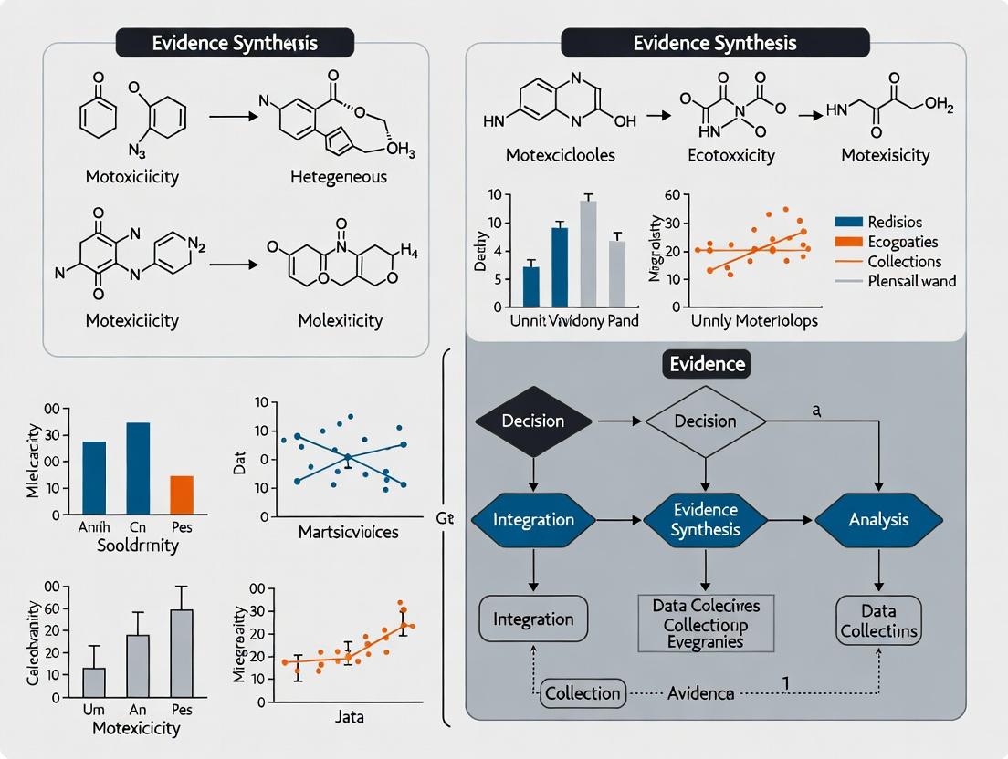
Visualizing Workflows and Pathways
Workflow for Integrating Heterogeneous Data into Evidence Synthesis
Title: Decision Workflow for Evidence Synthesis of Heterogeneous Data
HeMHAS Experimental Concept and Data Integration
Title: HeMHAS Multi-Habitat Assay Concept and Data Flow
The Researcher's Toolkit: Essential Reagents & Materials
The following table details key solutions and materials critical for conducting ecotoxicological experiments that account for heterogeneity, particularly in behavioral and multi-habitat assays.
| Research Reagent / Material | Primary Function in Context of Heterogeneity | Notes on Use & Standardization |
|---|---|---|
| Reference Toxicant (e.g., KCl, CuSO₄) | Controls for population sensitivity variability. Regular tests with a reference toxicant ensure the baseline response of your test organism population is within an expected range, separating inherent biological variability from treatment effects. | Use a standardized solution. Run with each batch of organisms. Record LC50/EC50 and compare to historical lab control charts. |
| Behavioral Assay Dye (e.g., non-toxic UV tracer) | Visualizes water flow and mixing in multi-chamber systems like HeMHAS. Confirms the establishment and maintenance of intended chemical gradients between compartments, a foundational requirement for non-forced exposure tests [1]. | Must be rigorously tested for no behavioral effect on test species. Use with a fluorometer for quantitative mapping of gradient stability. |
| Standardized Reconstituted Water (e.g., ASTM, OECD) | Minimizes heterogeneity from water chemistry. Provides a consistent ionic background, reducing uncontrolled interaction between the test chemical and variable natural water constituents that can affect bioavailability and toxicity. | Prepare in large batches for a single study. Characterize pH, hardness, alkalinity. Contrast results with tests in natural waters to assess interaction heterogeneity. |
| Automated Tracking Software (e.g., EthoVision, idTracker) | Quantifies behavioral heterogeneity. Converts organism movement (speed, location, turning) into high-dimensional data, allowing detection of subtle sub-lethal stress responses and preferences that simple count-based endpoints miss [1]. | Requires high-contrast video. Set thresholds consistently. Calibrate for chamber size. Outputs should include raw movement paths for re-analysis. |
| Cryopreserved Cell Lines or Clone Cultures | Reduces genetic heterogeneity for mechanistic in vitro studies. Using standardized, genetically identical biological material isolates chemical response from genetic variability, clarifying signal in pathway-based assays. | Document passage number and culture conditions. Use appropriate positive and solvent controls. Recognize this removes ecological realism for the sake of mechanistic clarity. |
Technical Support Center: Troubleshooting Heterogeneous Ecotoxicity Data
Welcome to the Technical Support Center for Evidence Synthesis Research. This resource is designed for researchers and scientists navigating the challenges of integrating heterogeneous ecotoxicity data. The following guides and FAQs address common issues encountered during experimental work and data synthesis, framed within the critical context of managing variability for robust evidence-based conclusions [5] [6].
Frequently Asked Questions (FAQs)
Q1: Why do my ecotoxicity test results (e.g., LC50) show high variability when repeating tests with the same chemical and species? A1: Unexplained variability in dose metrics like LC50 is a common and often under-characterized issue. Variability can stem from undocumented influences of "toxicity modifying factors" and model assumptions [7]. Key sources include:
- Test Organism Characteristics: Differences in body size, lipid content, and life stage between batches of test organisms can significantly alter toxicokinetics (how the chemical is absorbed, distributed, metabolized, and excreted) [7].
- Exposure Conditions: Factors such as exposure duration, water chemistry (e.g., pH, organic carbon), and temperature are not always sufficiently controlled or reported, impacting the bioavailability and effect of the chemical [7].
- Mode of Toxic Action: The fundamental relationship between external concentration and internal critical body residue (CBR) differs among toxic mechanisms (e.g., narcosis vs. reactive toxicity). Standard tests rarely validate the assumed mode of action, introducing uncertainty [7]. Troubleshooting Step: Review and rigorously standardize your test protocol. Document organism source, size range, and lipid content if possible. Characterize and report all water chemistry parameters. Consider if the chemical's mode of action is known and if your test duration is appropriate for that mechanism.
Q2: How reliable are extrapolations from a standard laboratory single-species test (e.g., Daphnia magna) for predicting effects on entire ecosystems? A2: This is a fundamental challenge in ecological risk assessment (ERA). While standard tests are reproducible, their relevance to protecting ecosystems is limited by the "mismatch" between measurement and assessment endpoints [6]. The primary issue is the disparity between what is measured (e.g., survival of an individual in a lab) and what society aims to protect (e.g., biodiversity, ecosystem function) [6]. Single-species tests:
- Miss ecological interactions (e.g., predator-prey dynamics, competition) that can amplify or mitigate stress.
- Do not account for recovery processes at the population or community level after exposure ceases.
- Use species chosen for culturing ease, which may not be the most sensitive in a real ecosystem [8]. Troubleshooting Step: For screening, use standard tests but acknowledge their conservatism and uncertainty. For higher-tier assessment when risks are indicated, advocate for or employ microcosm/mesocosm tests or mechanistic effect models that can incorporate ecological complexity and interactions [6].
Q3: I have a data-poor chemical. What are my best options for estimating ecotoxicity effects for a comparative assessment? A3: You can employ a tiered strategy that combines available data with in silico predictions, as recommended by next-generation frameworks [9] [10]. The goal is to avoid neglecting data-poor chemicals, which biases comparative decisions. A practical workflow is:
- Search for Analogues: Use read-across to borrow data from chemicals with similar structures and known effects.
- Apply In Silico Models: Use Quantitative Structure-Activity Relationship (QSAR) models to predict baseline toxicity [10].
- Use Extrapolation Factors: Apply intra- and inter-species extrapolation factors to convert available acute data to chronic estimates, or to estimate values for untested species [10]. For example, a fixed concentration-response slope can be assumed to derive an EC10 from an EC50 [10].
- Build a Hybrid SSD: Construct a Species Sensitivity Distribution (SSD) using any available measured data points and fill gaps with cautiously selected predicted values. Always quantify and report the associated uncertainty [10].
Q4: How can I integrate data from different sources (e.g., in vitro HTS, in vivo animal tests, omics data) to identify a chemical's mechanism of action? A4: Heterogeneous data integration is key for mechanism elucidation and requires unsupervised computational methods. Supervised methods need pre-defined categories, but novel mechanisms require unsupervised approaches. A robust method is:
- Generate Multi-Dimensional Profiles: Use assays with different endpoints (e.g., cell viability, caspase-3/7 activation for apoptosis, high-throughput transcriptomics) across multiple cell types or test systems [11].
- Apply Unsupervised Clustering: Use algorithms like Growing Self-Organizing Maps (GSOM) or multiple kernel learning to group chemicals based on their integrated biological profiles without prior labeling [12] [13].
- Validate Cluster Quality: Use indices like Dunn's Index to assess the validity and separation of the identified clusters [11].
- Interpret Clusters: Chemicals clustering together are likely to share a similar mechanism of action (MoA). This hypothesis can then be tested with targeted follow-up experiments [11] [12].
Q5: What is the best way to visualize and communicate the multi-faceted hazard profile of a chemical when comparing alternatives? A5: Move beyond single metrics and use integrated visualization tools that represent multiple lines of evidence. The Toxicological Priority Index (ToxPi) is a powerful visualization framework recommended for alternatives assessment [5]. It:
- Creates a radial diagram where each "slice" represents a different hazard dimension (e.g., acute aquatic toxicity, chronic mammalian toxicity, bioaccumulation potential).
- The size of each slice is weighted by the importance and confidence of the data.
- The overall area of the chart provides an integrated visual hazard score for easy comparison between chemicals. This approach forces transparent consideration of all endpoint data and their uncertainties, supporting more informed and defensible decisions [5].
Experimental Protocol Guidance
Protocol 1: Quantitative High-Throughput Screening (qHTS) for Cytotoxicity and Apoptosis [11] Objective: To generate concentration-response profiles for a large compound library, screening for general cytotoxicity and specific induction of apoptosis. Key Steps:
- Cell Preparation: Plate adherent cell lines (e.g., HepG2, HEK293) at 1000-2000 cells/well in 1536-well plates. Allow 5-6 hours for attachment. Suspend cells (e.g., Jurkat) are dispensed just before compound addition.
- Compound Treatment: Using a pin tool, transfer compounds from a source plate (14 concentrations, typically from 0.5 nM to 92 μM) to the assay plate. Include controls: tamoxifen and staurosporine as positive controls for caspase activation, and DMSO as a vehicle control.
- Assay Incubation:
- Cell Viability (ATP content): Incubate with compound for 40 hours. Add a homogeneous ATP detection reagent (e.g., CellTiter-Glo), incubate, and measure luminescence.
- Caspase-3/7 Activation: Incubate with compound for 16 hours. Add Caspase-Glo 3/7 reagent, incubate at room temperature for 1 hour, and measure luminescence.
- Data Analysis: Normalize raw luminescence to vehicle (0%) and positive control (100%) values. Fit concentration-response curves for each compound and endpoint to derive potency (e.g., AC50) and efficacy values.
Protocol 2: Problem Formulation for Ecological Risk Assessment (ERA) [8] Objective: To establish the foundation and plan for an ERA, ensuring it is focused on relevant protection goals. Key Steps:
- Planning Dialogue: Risk assessors and managers agree on management goals (e.g., "protect aquatic community structure"), regulatory context, scope, and resources.
- Integrate Available Information: Compile data on the stressor (chemical properties, use patterns), potential exposure pathways, and available ecotoxicity effects data.
- Select Assessment Endpoints: Define the specific ecological entity (e.g., salmonid fish populations) and its valued attribute (e.g., reproductive success) to be protected.
- Develop a Conceptual Model: Create a diagram (see Diagram 1 below) linking the stressor sources to exposure routes and potential effects on assessment endpoints. This identifies key hypotheses and data gaps.
- Develop an Analysis Plan: Specify how data will be analyzed (e.g., hazard quotients, probabilistic models), the measures to be used (e.g., HC20 from an SSD), and how uncertainty will be addressed.
Data Variability and Integration Tables
Table 1: Influence of Toxicity Modifying Factors on Aquatic Toxicity Dose Metrics (LC50) [7] Model-based analysis showing how variability in organism and test conditions can affect reported toxicity values.
| Modifying Factor | Condition 1 | Condition 2 | Potential Impact on LC50 (Order of Magnitude) | Primary Influence |
|---|---|---|---|---|
| Hydrophobicity (log Kow) | Low (e.g., 1) | High (e.g., 6) | Up to 10³ | Toxicokinetics, Bioaccumulation |
| Exposure Duration | Acute (48-hr) | Chronic (Life-cycle) | 10¹ - 10² | Toxicokinetics, Toxicodynamics |
| Organism Lipid Content | Low (1%) | High (10%) | Up to 10¹ | Critical Body Residue (CBR), Partitioning |
| Mode of Toxic Action | Narcosis (Baseline) | Reactive Toxicity | Can vary significantly | Critical Body Residue (CBR) Level |
| Metabolic Capacity | No degradation | Rapid degradation | 10¹ - 10² | Internal Biologically Effective Dose |
Table 2: Characteristics of Ecological Risk Assessment (ERA) Across Tiers [6] Higher tiers reduce uncertainty and increase ecological relevance but require greater resources.
| Tier | Description | Risk Metric | Data & Resource Requirements | Pros & Cons |
|---|---|---|---|---|
| I (Screening) | Conservative analysis to "screen out" low-risk scenarios. | Hazard Quotient (HQ = Exposure/Effect). Compared to Level of Concern. | Minimal. Uses standard lab toxicity data (e.g., LC50) and generic exposure models. | Pro: Fast, inexpensive. Con: High uncertainty, may over-predict risk. |
| II (Refined) | Incorporates variability (e.g., species sensitivity) and probabilistic exposure. | Probability of exceeding an effects threshold. | Moderate. Requires species sensitivity distributions (SSDs) and probabilistic exposure modeling. | Pro: Quantifies risk probability. Con: Still relies on lab-to-field extrapolation. |
| III (Advanced) | Site-specific or population/community-level assessment. | Risk to population growth rate or community metrics. | High. May require field data, mesocosm studies, or complex mechanistic models. | Pro: High ecological relevance. Con: Resource-intensive, complex. |
| IV (Definitive) | Direct measurement in the field under realistic conditions. | Field-observed effects (e.g., species abundance, ecosystem function). | Very High. Long-term monitoring or large-scale field studies. | Pro: Most direct evidence. Con: Costly, time-consuming, confounded by multiple stressors. |
Visualizations: Workflows and Relationships
Diagram 1: Conceptual Model for Ecological Risk Problem Formulation [8]
Diagram 2: Unsupervised Integration of Heterogeneous Data for MoA Clustering [12] [13]
The Scientist's Toolkit: Essential Research Reagents & Materials
Table 3: Key Reagents and Materials for In Vitro Ecotoxicology and HTS Core components for setting up cell-based and high-throughput screening assays as described in the protocols.
| Item | Example/Description | Primary Function in Research | Reference |
|---|---|---|---|
| Cell Lines | HepG2 (human hepatoma), HEK293 (human kidney), SH-SY5Y (human neuroblastoma), Daphnia magna (crustacean) cultures. | Provide in vitro or in vivo test systems representing different tissues, species, and trophic levels for toxicity profiling. | [11] |
| qHTS Assay Kits | CellTiter-Glo (ATP viability), Caspase-Glo 3/7 (apoptosis), other pathway-specific luminescent/fluorescent kits. | Enable homogeneous, miniaturized, high-throughput measurement of specific cellular endpoints (viability, apoptosis, oxidative stress). | [11] |
| Microplate Readers | Luminescence/fluorescence-capable plate readers (e.g., ViewLux, EnVision). | Detect signals from assay kits in 96-, 384-, or 1536-well plate formats for high-throughput screening. | [11] |
| Standardized Test Media | OECD-recommended freshwater (e.g., ISO, EPA), marine, or soil media. | Ensure reproducibility and comparability of ecotoxicity tests across laboratories by controlling water/sediment chemistry. | [5] [8] |
| Reference & Control Compounds | Staurosporine, Tamoxifen, Potassium Dichromate, DMSO. | Serve as positive (known toxicant) and negative (vehicle) controls to validate assay performance and data normalization. | [11] |
| In Silico & NAM Tools | QSAR Toolboxes (e.g., OECD QSAR), ToxCast database, AOP-Wiki, microphysiological system (MPS) protocols. | New Approach Methodologies (NAMs) used for prediction (QSAR), screening (HTS), and mechanistic understanding (AOPs) to supplement or reduce traditional testing. | [9] |
Welcome to the Evidence Synthesis Technical Support Center
This guide provides troubleshooting support for researchers integrating heterogeneous ecotoxicity data. The historical reliance on endpoints like the No Observed Effect Concentration (NOEC) creates inconsistency in modern evidence synthesis and ecological risk assessment (ERA). Below, you will find solutions to common problems, framed within a thesis on advancing data harmonization and analysis.
Quick-Reference Table: Historical vs. Modern Ecotoxicity Endpoints
| Metric | Definition | Key Limitation for Evidence Synthesis | Preferred Modern Alternative |
|---|---|---|---|
| NOEC | Highest tested concentration with no statistically significant effect (p<0.05) compared to control [14] [15]. | Depends on arbitrary test concentrations; no confidence interval; misrepresents "no effect" [14] [16]. | ECx (e.g., EC10) [15] or Benchmark Dose (BMD) [16]. |
| LOEC | Lowest tested concentration with a statistically significant effect [14] [15]. | Same as NOEC; provides no information on the concentration-response relationship [14]. | Derived from a fitted concentration-response model. |
| MATC | Geometric mean of NOEC and LOEC [15]. | Inherits all flaws of its parent NOEC/LOEC values. | Not recommended; use model-derived estimates. |
| ECx | Concentration causing an x% effect (e.g., EC10) from a continuous model [15]. | Requires high-quality data with multiple concentrations for reliable fitting. | Considered a more robust and informative default [16]. |
Troubleshooting Guide: FAQs & Solutions
Issue Category 1: Handling Legacy Data & Inconsistent Endpoints
Problem: My meta-analysis includes studies that only report NOEC/LOEC. How can I use this data alongside studies reporting modern ECx values?
Solution: You cannot directly combine NOEC and ECx values statistically. Follow this workflow:
- Categorize & Segregate: Separate studies by endpoint type (NOEC/LOEC vs. ECx).
- Use Assessment Factors: For risk assessment, apply a larger assessment factor (e.g., 10 to 50) to a NOEC-based PNEC to account for its greater uncertainty before comparing it to an ECx-based PNEC [15].
- Sensitivity Analysis: Run your synthesis twice—once with all data (converting where possible) and once only with model-based endpoints (ECx/BMD)—to gauge the impact of legacy metrics.
Problem: A key regulatory document for my chemical only provides a MATC. How do I proceed?
Solution: The MATC is the geometric mean of the NOEC and LOEC. You can approximate a NOEC by dividing the MATC by √2 (approximately 1.414) [15]. Document this assumption clearly as a source of uncertainty in your analysis.
Issue Category 2: Dealing with Heterogeneous Data Quality
Problem: I have gathered ecotoxicity data from multiple sources (journals, regulatory dossiers, unpublished reports). How do I screen it for reliability?
Solution: Implement a structured data curation workflow, such as the Stepwise Information-Filtering Tool (SIFT) methodology used for the EnviroTox database [17].
- Step 1: Apply Acceptance Criteria. Use a checklist derived from regulatory guidelines [18]:
- Is the study on a whole, live organism?
- Is a concurrent control group reported?
- Is the exposure concentration and duration explicit?
- Is a calculable endpoint reported?
- Is the species verified?
- Step 2: Classify Studies. Label studies as "Accepted," "Rejected," or "Requiring Expert Judgment" [18].
- Step 3: Document. Maintain a transparent review summary for each study, noting reasons for inclusion/exclusion.
Data Curation and Screening Workflow for Ecotoxicity Studies
Problem: I am using the U.S. EPA's ECOTOX database and finding inconsistencies. What are common known issues?
Solution: Be aware of systemic data problems. For example, in water quality data, parameter codes for pH violations can be misapplied, leading to erroneous flags [19]. Always:
- Trace data to the primary source where possible.
- Consult EPA's "Known Data Problems" pages for your relevant program (e.g., Clean Water Act) [19].
- Use curated databases like EnviroTox, which applies uniform quality filters, as a more consistent source [17].
Issue Category 3: Modern Statistical Analysis & Model Fitting
Problem: My concentration-response data is messy (non-linear, bounded counts, low replicate count). What statistical model should I use?
Solution: Move beyond basic ANOVA. Use Generalized Linear Models (GLMs) or non-linear regression as your default [16].
- For binary data (e.g., mortality): Use a GLM with a logit or probit link function.
- For count data (e.g., offspring number): Use a GLM with a log link (Poisson or Negative Binomial distribution).
- For continuous data (e.g., growth): Use a non-linear model (e.g., 2-5 parameter logistic models).
- These methods allow you to estimate an ECx with confidence intervals directly, providing more information than a NOEC [14] [16].
Problem: I need to analyze a dataset with nested structures (e.g., multiple tests from the same lab). How do I account for this?
Solution: Use a mixed-effects model (a hierarchical GLM). This allows you to model the fixed effect of concentration while accounting for random variation from labs, species clones, or test batches [16]. This prevents pseudoreplication and gives more accurate confidence intervals.
Comparison of Legacy and Modern Statistical Analysis Pathways
Featured Experiment & Protocol: Integrating Heterogeneous Data for a Silver Nanoparticle (SNP) Case Study
Objective: To synthesize evidence on the aquatic toxicity of Silver Nanoparticles (SNPs) for a predictive risk assessment, despite heterogeneous data from studies using different endpoints (NOEC, EC50, LC50), species, and SNP characteristics.
Experimental Protocol: Evidence Synthesis Workflow
1. Problem Formulation & Data Mining:
- Define the assessment goal: e.g., "Derive a predicted no-effect concentration (PNEC) for SNPs in freshwater."
- Search multiple sources: curated databases (EnviroTox [17], ECOTOX [18]), regulatory filings, and peer-reviewed literature.
- Use broad search terms: "silver nanoparticle," "aquatic toxicity," "Daphnia," "fish," "algae," "chronic," "acute."
2. Data Curation & Harmonization (Critical Step):
- Extract Data: For each study, record: species, endpoint (NOEC, EC50, etc.), endpoint type (mortality, growth, reproduction), exposure time, SNP size, coating, and synthesis method [20].
- Apply Quality Filters: Use the SIFT criteria [17] or EPA guidelines [18] to accept/reject studies.
- Harmonize Endpoints:
3. Data Analysis & Modeling:
- Species Sensitivity Distribution (SSD): Fit a statistical distribution (e.g., log-normal) to the most sensitive chronic endpoint for each species.
- Calculate HC5: Derive the Hazardous Concentration for 5% of species (HC5) from the SSD. Often used as a PNEC.
- Account for Nano-Specific Properties: Use a QSAR-perturbation model if data allows, which can predict toxicity based on SNP size, coating, and test conditions [21].
- Statistical Tools: Perform all analyses in R using packages like
drc(dose-response curves),ssdtools(SSDs), andlme4(mixed-effects models) [16].
4. Risk Characterization & Reporting:
- Compare the PNEC to environmentally relevant SNP concentrations.
- Transparently report all data sources, curation decisions, conversion factors, and model assumptions.
The Scientist's Toolkit: Research Reagent Solutions
| Tool/Resource | Function in Evidence Synthesis | Key Consideration |
|---|---|---|
| EnviroTox Database [17] | Curated aquatic toxicity database with quality-controlled data. Provides tools for PNEC calculation and chemical toxicity distributions. | Ideal for finding reliable, pre-filtered data. Superior for consistency over raw database searches. |
| ECOTOX Knowledgebase [18] | EPA's comprehensive ecotoxicity database. Useful for broad, initial data gathering. | Requires rigorous post-hoc curation by the user; check for "Known Data Problems" [19]. |
| R Statistical Software [16] | Open-source platform for advanced statistical analysis (GLMs, SSDs, nonlinear fitting). Essential for modern dose-response modeling. | Steep learning curve but necessary for moving beyond NOEC/LOEC. Use established ecotoxicology packages. |
| OECD Guidance No. 54 (Under Revision) [16] | Future international guideline on statistical analysis of ecotoxicity data. | The 2026 revision is expected to formally deprecate NOEC and endorse regression-based methods. |
| QSAR-Perturbation Models [21] | Computational tool to predict nanoparticle ecotoxicity under varying experimental conditions (size, coating, organism). | Crucial for interpreting heterogeneous SNP data and filling data gaps without new animal testing. |
The Implications of Heterogeneity for Evidence Synthesis and Risk Assessment
In evidence synthesis for environmental and human health risk assessment, heterogeneity—the variability in effect sizes or outcomes across different studies—is not merely a statistical nuisance but a central feature containing critical scientific information [22]. This variability arises from differences in biological systems, experimental designs, exposure parameters, and measured endpoints [23]. For professionals synthesizing ecotoxicity data, effectively handling this heterogeneity is paramount to producing reliable, actionable conclusions for chemical safety decisions [24]. This technical support center provides targeted guidance, protocols, and troubleshooting advice to help researchers navigate the specific challenges posed by heterogeneous data streams in evidence synthesis and ecological risk assessment [22] [23].
Frequently Asked Questions (FAQs) on Heterogeneity
Q1: What are the primary sources of heterogeneity in ecotoxicity evidence synthesis? A1: Heterogeneity in ecotoxicity meta-analyses typically stems from three core areas:
- Biological and Ecological Variance: Differences in species sensitivity, life stages, trophic levels (e.g., producers vs. consumers), and genetic variability contribute to true biological variation in responses to a stressor [23].
- Methodological Diversity: Variations in experimental design (e.g., lab vs. field studies), exposure durations (acute vs. chronic), measured endpoints (e.g., LC50, NOEC, growth inhibition), and laboratory protocols introduce systematic differences [24] [22].
- Statistical and Sampling Error: Inherent random error from small sample sizes, particularly in single-arm studies or those reporting rare events, can manifest as observed heterogeneity [22].
Q2: Why is the choice of a heterogeneity variance estimator (τ²) critical, and which one should I use? A2: The estimator for between-study variance (τ²) directly influences the weights assigned to individual studies in a random-effects meta-analysis and the width of confidence and prediction intervals. Research indicates no single estimator performs best universally; performance depends on the number of studies, outcome type (continuous/binary), and presence of rare events [22]. A 2025 simulation study found all common estimators can be imprecise, especially with few studies, and often underestimate true heterogeneity [22]. It is therefore recommended to compare multiple estimators (e.g., DerSimonian-Laird, Paule-Mandel, restricted maximum likelihood) and incorporate this analysis into sensitivity analyses rather than relying on a single default method [22].
Q3: How can I proceed with evidence synthesis for risk assessment when faced with high and unexplained heterogeneity? A3: High heterogeneity (e.g., high I² statistic) does not invalidate a synthesis but requires careful interpretation and transparent reporting.
- Investigate Sources: Use subgroup analysis or meta-regression to explore if factors like taxonomic group or exposure duration explain the variance [23].
- Employ More Appropriate Models: Consider switching from an aggregate data meta-analysis to other models. For ecological risk, Species Sensitivity Distribution (SSD) modeling is a specialized framework designed to handle interspecies variability by fitting a statistical distribution to toxicity data, estimating concentrations hazardous to a specified fraction of species (e.g., HC-5) [23].
- Qualitative Integration: In cases of extreme heterogeneity, a quantitative summary may be misleading. Shift to a systematic review with qualitative, narrative synthesis and explicit weight-of-evidence evaluation, clearly describing the inconsistency in the evidence base [24].
Q4: What are the best practices for transparently reporting heterogeneity in a meta-analysis or systematic review? A4: Transparency is key for credibility and reproducibility.
- Pre-specify Methods: State in your protocol how you will assess and investigate heterogeneity (statistics, subgroup analyses).
- Report Multiple Metrics: Present both τ² (absolute measure) and I² (relative measure) with their confidence intervals [22].
- Conduct and Report Sensitivity Analyses: Demonstrate how key conclusions change under different heterogeneity estimators or statistical models [22].
- Interpret in Context: Discuss the potential biological and methodological reasons for the observed heterogeneity and its implications for the certainty of the overall evidence and for generalizing conclusions [24].
Technical Support: Troubleshooting Common Scenarios
Scenario 1: Low Precision or Zero Estimate for Heterogeneity Variance (τ²)
Problem: Your random-effects meta-analysis yields a τ² estimate of zero or an implausibly small value, despite clear visual or subject-matter indications of between-study differences.
| Potential Cause | Diagnostic Check | Corrective Action |
|---|---|---|
| Insufficient number of studies | Check if k < 10. Meta-analyses with few studies have very low power to detect heterogeneity [22]. |
Do not simplistically revert to a fixed-effect model. Acknowledge the limitation. Consider presenting prediction intervals from a random-effects model regardless, as they better represent uncertainty for new studies. |
| Use of an estimator prone to underestimation | The common DerSimonian-Laird (DL) estimator is known to underestimate τ², especially with binary outcomes [22]. | Re-estimate τ² using alternative estimators (e.g., Paule-Mandel (PM), Restricted Maximum Likelihood (REML)). Report results from multiple estimators as a sensitivity analysis [22]. |
| Overly conservative outcome measure | Assess if the chosen effect size metric (e.g., risk difference) is less prone to show variability than others (e.g., log odds ratio). | Consider the biological rationale for the effect measure. Re-analysis with a different, justifiable metric may be informative. |
Systematic Troubleshooting Protocol [25]:
- Identify: The problem is an unexpectedly low τ² estimate.
- List Explanations: Few studies; inappropriate estimator; choice of effect measure.
- Collect Data: Record the number of studies (
k). Note the estimator used and the type of outcome data. - Eliminate/Test: Run analyses using at least two alternative τ² estimators (e.g., PM, REML). Compare results.
- Check with Experimentation: If possible, explore the impact using a different, biologically plausible effect size metric.
- Identify Cause: Conclude based on which change most substantially alters τ². Document all steps and decisions.
Scenario 2: Overfitting or Poor Extrapolation in Species Sensitivity Distribution (SSD) Models
Problem: Your SSD model, developed from laboratory toxicity data, fails validation or produces unrealistic hazardous concentration (e.g., HC-5) estimates when applied to new chemicals or field data.
| Potential Cause | Diagnostic Check | Corrective Action |
|---|---|---|
| High uncertainty due to small or biased dataset | Evaluate if data spans few taxonomic groups or is clustered around a single species or test type. | Incorporate data from curated databases (e.g., EPA ECOTOX) to increase taxonomic breadth [23]. Use bootstrapping to quantify uncertainty in the HC-5 estimate. Clearly state the model's domain of applicability. |
| Poor model choice for the data distribution | Visually inspect the fit of the chosen distribution (e.g., log-normal, log-logistic) to the data points. | Test the goodness-of-fit for different statistical distributions. Consider using robust regression techniques or model averaging if no single distribution fits well. |
| Ignoring important covariates | Check if species traits (e.g., trophic level, body size) or chemical properties explain residual variance. | Develop hierarchical or mixture SSD models that account for taxonomic groups or chemical classes. A 2025 study demonstrated the value of class-specific SSD models for chemicals like personal care products [23]. |
Detailed Experimental and Analytical Protocols
Purpose: To determine the sensitivity of your meta-analysis conclusions to the choice of τ² estimator.
Materials: Statistical software capable of meta-analysis (R, Stata, Python). Dataset of study effect sizes and their variances.
Methodology:
- Perform Base Analysis: Conduct the random-effects meta-analysis using your software's default estimator (often DerSimonian-Laird).
- Select Alternative Estimators: Choose at least two additional estimators known to have different properties. Recommended candidates include:
- Paule-Mandel (PM): Good performance with binary data.
- Restricted Maximum Likelihood (REML): An iterative, likelihood-based method.
- Sidik-Jonkman (SJ): Can be more stable with few studies.
- Re-run Analyses: Perform separate meta-analyses identical in all respects except for the τ² estimator.
- Extract Key Outputs: For each analysis, record: τ² estimate, I² statistic, the overall effect estimate (θ), and its 95% confidence and prediction intervals.
- Synthesis and Reporting: Present results in a comparative table. Discuss if and how the central conclusion or the range of plausible effects (prediction interval) changes across estimators.
Purpose: To estimate the concentration of a chemical that is hazardous to 5% of species (HC-5) by modeling the distribution of species sensitivities.
Materials: Curated ecotoxicity dataset (e.g., from EPA ECOTOX), statistical software (R, Python with SciPy), SSD modeling platform (e.g., OpenTox SSDM).
Methodology:
- Data Curation & Selection:
- Compile acute (e.g., LC50/EC50) or chronic (NOEC/LOEC) toxicity values for the target chemical.
- Ensure data spans multiple taxonomic groups (e.g., algae, invertebrates, fish) for ecological relevance.
- For each record, use the most sensitive reported endpoint per species.
- Data Transformation: Log-transform all toxicity values (typically base 10) to approximate a normal distribution.
- Distribution Fitting:
- Fit several theoretical distributions (e.g., log-normal, log-logistic, Burr Type III) to the log-transformed data.
- Use maximum likelihood estimation or rank-based methods for parameter estimation.
- Model Selection & Validation:
- Compare fitted models using goodness-of-fit criteria (e.g., Kolmogorov-Smirnov test, AIC).
- Use bootstrapping (e.g., 1000 iterations) to estimate the confidence interval around the HC-5 and other percentiles.
- Interpretation & Reporting:
- Report the selected distribution, its parameters, the HC-5 with its confidence interval, and the species used.
- Clearly state the model's limitations and applicable domain (e.g., "based on freshwater aquatic species").
Decision Workflow for Heterogeneous Ecotoxicity Data Synthesis
The Scientist's Toolkit: Essential Research Reagent Solutions
| Item/Category | Primary Function in Ecotoxicity Evidence Synthesis | Example & Notes |
|---|---|---|
| Meta-Analysis Software Packages | Statistical computation for pooling effects, estimating heterogeneity, and generating forest plots. | R packages (metafor, meta), Stata (metan), RevMan. Essential for implementing and comparing different τ² estimators [22]. |
| Curated Ecotoxicity Databases | Source of standardized, quality-controlled experimental toxicity data across species and endpoints. | U.S. EPA ECOTOX Knowledgebase. Critical for building robust Species Sensitivity Distribution (SSD) models [23]. |
| SSD Modeling Tools | Specialized software for fitting statistical distributions to toxicity data and deriving HC-p values. | OpenTox SSDM platform, R package fitdistrplus. Facilitates model fitting, validation, and visualization [23]. |
| Systematic Review Management Software | Aids in screening references, data extraction, and managing the review process to reduce bias. | Rayyan, Covidence, DistillerSR. Supports transparent and reproducible evidence gathering per EFSA/IRIS frameworks [24]. |
| Reference Management Software | Organizes literature, formats citations, and ensures traceability. | Zotero, EndNote, Mendeley. Fundamental for handling large bibliographies in systematic reviews. |
| Biomarker Assay Kits (e.g., ELISA) | Generates standardized mechanistic or apical endpoint data for experimental studies. | Quantikine ELISA Kits (R&D Systems). Used to measure specific proteins (e.g., stress biomarkers) in in-vivo or in-vitro toxicity studies, providing high-quality data for synthesis [26]. |
Species Sensitivity Distribution (SSD) Model Workflow
Effectively managing heterogeneity is fundamental to robust evidence synthesis in ecotoxicology and risk assessment. Key strategies include moving beyond a single statistical estimator to compare multiple methods, transparently investigating and reporting the sources of variability, and selecting the synthesis framework—be it meta-analysis, SSD modeling, or qualitative weight-of-evidence—that best aligns with the nature and patterns of the heterogeneous data [24] [22] [23]. By adopting the systematic troubleshooting approaches and detailed protocols outlined in this guide, researchers can enhance the reliability, transparency, and regulatory utility of their assessments in the face of complex, real-world data.
Advanced Methods for Harmonizing and Analyzing Heterogeneous Ecotoxicity Data
In evidence synthesis research for ecotoxicology, data heterogeneity is the rule, not the exception. Traditional analysis of variance (ANOVA) operates under assumptions of normality and homoscedasticity (constant variance) that are frequently violated by toxicological data, where variance often changes with dose and responses can be binary, count, or continuous [27]. This mismatch can lead to biased conclusions and a loss of regulatory trust. Modern statistical frameworks, specifically Generalized Linear Models (GLMs) and dose-response modeling, provide the necessary flexibility to model data according to its true distribution and variance structure. This transition is critical for deriving robust, reproducible benchmarks—like the Benchmark Dose (BMD)—from heterogeneous evidence streams, forming the analytical core of a thesis dedicated to improving ecological risk assessment.
Technical Support Center: Troubleshooting Guides & FAQs
This section addresses common analytical challenges encountered when implementing GLMs and dose-response models for heterogeneous data.
Troubleshooting Guide: Common Issues & Solutions
Table 1: Troubleshooting Common Statistical Issues in Dose-Response Analysis
| Problem Symptom | Likely Cause | Diagnostic Check | Recommended Solution |
|---|---|---|---|
| Non-normality of residuals | Response data may be intrinsically non-normal (e.g., counts, percentages). | Histogram or Q-Q plot of residuals; Shapiro-Wilk test. | Use a GLM with an appropriate non-normal family (e.g., binomial for proportions, Poisson for counts) [28]. |
| Variance heterogeneity (Heteroscedasticity) | Variance changes with the mean response (e.g., smaller variance at high-effect doses) [27]. | Plot residuals vs. fitted values; Breusch-Pagan test. | Apply variance-stabilizing transformation (e.g., Box-Cox) or use a GLM that models the mean-variance relationship directly [27]. |
| Overdispersion in Binomial/Poisson GLMs | Observed variance > variance predicted by the model. | Check residual deviance/degrees of freedom >> 1. | Switch to a quasi-likelihood model (e.g., quasibinomial) or a negative binomial GLM. |
| Model fitting failure or instability | Poor starting values for parameters; model mis-specification. | Error messages; parameter estimates at boundaries. | Use built-in self-starting functions; simplify the model; scale dose variable [29]. |
| Inaccurate confidence intervals for BMD | Assumption of constant standard deviation is violated [30]. | Compare residual spread across doses. | Implement a hybrid BMD method that accounts for a heterogeneous variance structure [30]. |
Frequently Asked Questions (FAQs)
Q1: When should I definitely choose a GLM over a traditional ANOVA? Use a GLM when your response data is not continuous and normal. This includes binary outcomes (dead/alive), count data (number of offspring), and proportions (percent immobilized). GLMs directly model these data types using the correct statistical distribution (binomial, Poisson, etc.), preventing the invalid inferences that can arise from applying ANOVA to such data [28].
Q2: My dose-response data shows unequal variance across doses. Can I just use a data transformation? While transformations (like log or square root) can sometimes stabilize variance for simple linear regression, they are often inappropriate for nonlinear dose-response modeling as they can distort the underlying S-shaped relationship [27]. A superior approach is to use a statistical model that explicitly accounts for variance heterogeneity. Recent advances extend methods like the hybrid Benchmark Dose (BMD) approach to incorporate dose-dependent variance, leading to less biased and more reliable safety estimates [30].
Q3: How do I handle a dataset where there is almost no response at low doses, but variance collapses at high, toxic doses? This pattern is common in sublethal toxicity tests [27]. A two-pronged strategy is effective: 1) Model the mean using a standard dose-response curve (e.g., a 4-parameter log-logistic model). 2) Model the variance separately, allowing it to be a function of the dose or the predicted mean response. This joint modeling, possible in advanced packages, correctly weights observations and provides valid confidence intervals.
Q4: I'm getting a good fit with my dose-response model, but how do I visually communicate the result and the BMD?
Always plot the raw data alongside the fitted curve. For binary data, plot the observed proportions. Use the fitted model to predict a smooth curve. To display the BMD and its lower confidence limit (BMDL), add vertical lines to the dose axis. In ggplot2, ensure you are using the correct link function (e.g., link="probit") and, for binomial data, specify the weights argument if using a proportion/weights format [31]. Avoid using the inverse link for a probit model, as this will misrepresent the relationship.
Q5: What are the key steps for a rigorous dose-response analysis workflow? A robust workflow involves: 1) Exploratory Data Analysis (visualize variance patterns, identify outliers). 2) Model Selection (choose a suitable mean function from families like log-logistic or Weibull [29]). 3) Model Fitting & Validation (fit model, check residual plots, assess overdispersion). 4) Inference (calculate EC/LC values or BMD/BMDL with confidence intervals). 5) Sensitivity Analysis (test robustness to model choice and variance assumptions).
Experimental Protocols & Methodologies
Protocol 1: Correcting for Non-Normality and Variance Heterogeneity in Sublethal Endpoints Based on the method by Ritz and Vander Vliet (2009) [27]. Objective: To derive accurate ECx estimates from continuous toxicity data violating standard regression assumptions.
- Data Collection: Obtain quantitative sublethal response data (e.g., growth, reproduction) across a minimum of 5-6 concentration levels with replicates.
- Initial Diagnosis: Fit a preliminary nonlinear model (e.g., log-logistic). Plot residuals versus fitted values to identify variance heterogeneity (often a "funnel" shape).
- Application of Box-Cox Transformation: If variance changes systematically but residuals are roughly normal, apply a Box-Cox power transformation to the response variable to stabilize variance across the dose range. The power parameter (λ) is estimated from the data.
- Model Refitting: Refit the nonlinear dose-response model to the transformed data. Alternatively, if the data are counts, specify a Poisson distribution within a GLM framework, which inherently accounts for mean-variance relationships.
- Endpoint Calculation: Calculate the desired effective concentration (e.g., EC50) from the final model. Confidence intervals derived from this model will be more reliable than those from a model ignoring variance issues.
Protocol 2: Hybrid Benchmark Dose (BMD) Estimation with Heterogeneous Variance Based on the hybrid method extension by Baalkilde et al. (2025) [30]. Objective: To estimate a BMD and its lower confidence limit (BMDL) for continuous data where the standard deviation varies with dose.
- Model Specification: Define a two-component model: a) a mean function (e.g., a polynomial or Hill model), and b) a variance function (e.g., modeling log(SD) as a linear function of dose or the mean).
- Parameter Estimation: Use maximum likelihood estimation to jointly fit the mean and variance model parameters to the experimental data.
- BMD Derivation: Define the BMD as the dose corresponding to a specified Benchmark Response (BMR), such as a 10% reduction from the background mean. Calculate this using the fitted mean model.
- Uncertainty Quantification: Compute the BMDL using a likelihood profiling approach that accounts for the uncertainty in both the mean and variance parameters. This contrasts with traditional methods that assume constant variance.
- Validation: Compare the coverage probability of the BMDL confidence interval from this method against the traditional method via simulation; the heterogeneous variance method should maintain coverage closer to the nominal (e.g., 95%) level.
Visualizing Analytical Workflows and Relationships
The Scientist's Toolkit: Essential Research Reagent Solutions
Table 2: Key Software, Packages, and Statistical Tools
| Tool/Reagent | Primary Function | Application in Analysis | Key Reference/Resource |
|---|---|---|---|
| R Statistical Environment | Open-source platform for statistical computing and graphics. | Core environment for implementing GLMs, dose-response models, and specialized BMD analysis. | [29] |
drc Package (R) |
Flexible infrastructure for fitting and analyzing dose-response curves. | Provides built-in models (log-logistic, Weibull, etc.), model averaging, and EC/LC calculation [29]. | [29] |
ggplot2 & Lets-Plot |
Grammar of Graphics-based plotting systems for R and Python. | Creates publication-quality visualizations of raw data, fitted curves, and confidence intervals [31] [32]. | [31] [32] |
| Box-Cox Transformation | A family of power transformations to stabilize variance and induce normality. | Corrects variance heterogeneity in continuous data prior to nonlinear regression [27]. | [27] |
| Hybrid BMD Method (Extended) | A statistical procedure for estimating the dose causing a low-level adverse effect. | The preferred method for continuous data, especially when extended to model heterogeneous variance for unbiased BMDL estimates [30]. | [30] |
| ColorBrewer Palettes | Sets of color schemes designed for clarity and accessibility in data visualization. | Used to distinguish treatment groups or represent sequential data on plots, ensuring interpretability [33]. | [33] |
| Quasi-Likelihood Models | Extension of GLMs to handle over- or under-dispersion. | Provides correct inference when the variance of count or proportion data exceeds the theoretical model variance. | [28] |
Technical Support Center: Troubleshooting SSDs in Evidence Synthesis Research
This technical support center assists researchers in developing and applying Species Sensitivity Distributions (SSDs) and risk curves, specifically within the context of synthesizing heterogeneous ecotoxicity data for evidence-based environmental risk assessment. The following guides address common methodological challenges, data integration issues, and interpretation problems.
Frequently Asked Questions (FAQs) & Troubleshooting
Q1: My dataset for a chemical includes toxicity values from diverse test species, endpoints (e.g., LC50, NOEC), and exposure durations. How do I create a coherent SSD from this heterogeneous data? A: Heterogeneity is a major challenge in evidence synthesis. To build a statistically valid SSD, you must first standardize and tier your data.
- Primary Action: Separate your data into acute (short-term, often lethal) and chronic (long-term, sub-lethal) datasets. An SSD should be constructed using data of the same type and severity [34]. For deriving a Predicted No-Effect Concentration (PNEC), chronic data is preferred.
- Data Selection Rule: For each species, select the most sensitive, reliable endpoint (e.g., the lowest NOEC for chronic data) to represent that species in the distribution [34].
- Minimum Data Requirements: Ensure your dataset meets taxonomic breadth requirements. A robust SSD typically requires a minimum of 7 species, encompassing at least 3 fish species, 3 invertebrate species, and 1 algal or aquatic plant species [34].
- Troubleshooting Tip: If chronic data is insufficient, you may use an acute SSD-derived value (like the HC5) and apply an appropriate Assessment Factor (AF) to extrapolate to a chronic protection level, acknowledging the increased uncertainty [34].
Q2: I have compiled toxicity data, but the statistical software fails to fit a distribution, or the fit is poor. What are the likely causes and solutions? A: Poor model fit often stems from inadequate data structure or true bimodality in species sensitivities.
- Common Cause 1: Insufficient or Clustered Data. A dataset with fewer than 7 species or one lacking representation across taxonomic groups may not form a recognizable statistical distribution.
- Solution: Expand your literature search to include more species from underrepresented groups (e.g., amphibians, sediment-dwelling organisms) [34].
- Common Cause 2: Bimodal Sensitivity Distributions. For chemicals with a specific mode of action (e.g., insecticides targeting acetylcholinesterase), sensitivities may cluster into two distinct groups (e.g., very sensitive arthropods vs. less sensitive fish and plants) [35] [34].
- Solution: Do not force a single distribution. Investigate if the data forms two logical groups. Advanced SSD tools allow fitting multiple distributions or using bimodal models to better characterize this pattern [34].
- Goodness-of-Fit Check: Always perform graphical and statistical (e.g., Anderson-Darling test) assessments to ensure the fitted model adequately describes your data [35] [34].
Q3: How do I interpret and use the HC5 value derived from my SSD in a real-world risk assessment? A: The Hazardous Concentration for 5% of species (HC5) is a key output but is not directly the "safe" threshold.
- Interpretation: The HC5 is the concentration estimated to affect 5% of species in the constructed SSD model. It is a statistical estimate with associated confidence intervals [35] [36].
- Risk Assessment Application: For screening-level assessment, the HC5 can be used directly as a benchmark value. A measured environmental concentration (MEC) exceeding the HC5 indicates potential risk. For a more protective Predicted No-Effect Concentration (PNEC), the HC5 is often divided by an Assessment Factor (AF), typically between 1 and 10, to account for uncertainties extrapolating from lab to field and from limited species to entire ecosystems [34] [36].
- From HC5 to Eco-TTC: In evidence synthesis, HC5 values for many chemicals can be aggregated to establish Ecological Thresholds of Toxicological Concern (Eco-TTCs) for chemical classes. This provides a screening-level threshold for data-poor chemicals based on the probability distribution of HC5 or PNEC values for similar compounds [35].
Q4: My goal is to assess the risk of a chemical mixture or a single chemical exposed to a multi-stress environment. Can SSDs handle this? A: Yes, the SSD framework can be extended to multi-stressor assessments through the concept of the Potentially Affected Fraction (PAF).
- Concept: For each stressor (e.g., Chemical A, Chemical B, increased temperature), a separate SSD is built. For a given exposure level, each SSD predicts the fraction of species affected (PAF) [36].
- Integration for Mixtures: The overall risk from multiple stressors can be estimated by combining the individual PAFs, resulting in a multi-stressor PAF (msPAF), which represents the total fraction of species affected by one or more of the stressors [36].
- Critical Consideration: This approach assumes independent action of stressors. Validation for specific interactive effects (synergy, antagonism) is an area of ongoing research and requires careful interpretation.
Q5: What are the main sources of uncertainty in an SSD-based risk assessment, and how can I quantify or report them? A: Transparency about uncertainty is crucial in evidence synthesis. Key sources include:
- Data Uncertainty: Limited number of species, lack of sensitive taxa, variability in test protocols, and data quality [34] [37].
- Model Uncertainty: Choice of statistical distribution (e.g., log-normal, log-logistic) and the fit of the model to the data [38] [34].
- Ecological Uncertainty: The degree to which a laboratory-derived SSD based on standard test species represents the sensitivity of a complex, adaptive field community [36].
- Reporting Best Practice: Always report confidence intervals around the HC5 (or other HCx) estimate. Clearly document your data selection criteria, the taxonomic composition of your dataset, the statistical model used, and any assessment factors applied in deriving a final protective value [34] [37].
Core Experimental & Computational Protocols
Protocol 1: Building a Standard SSD from Heterogeneous Ecotoxicity Data This protocol synthesizes guidance from Health Canada and the EPA for creating a defensible SSD [38] [34].
Data Compilation & Curation:
- Search: Conduct a systematic literature review using keywords (e.g., "[chemical name]" AND "toxicity" AND "LC50/NOEC/EC50") across scientific databases.
- Screen & Filter: Include only peer-reviewed studies with reliable, well-described methods. Exclude studies with major flaws.
- Standardize: Convert all effect concentrations (e.g., LC50, NOEC) to a consistent molar unit (e.g., µmol/L) using molecular weight [35].
- Categorize: Split data into acute and chronic sets. For chronic SSDs, use endpoints like growth, reproduction, or survival over full life-cycles.
Data Selection for SSD Input:
- For each unique species, identify the most sensitive, high-quality endpoint from the appropriate (acute/chronic) dataset.
- Apply a minimum data requirement: Aim for at least 7 species covering a minimum of 3 fish, 3 invertebrates, and 1 algae/plant species [34].
- Log-transform the selected toxicity values (e.g., log10(LC50)).
Distribution Fitting & HC5 Estimation:
- Use dedicated software (e.g., EPA SSD Toolbox [38], R package
ssdtools[34]). - Fit several plausible statistical distributions (e.g., normal, logistic, Gumbel) to the log-transformed data.
- Perform goodness-of-fit tests (e.g., Anderson-Darling) to select the most appropriate model.
- Calculate the HC5 (the 5th percentile of the fitted distribution) and its 95% confidence interval from the selected model.
- Use dedicated software (e.g., EPA SSD Toolbox [38], R package
Derivation of a Protective Concentration (PNEC):
- For a chronic SSD based on long-term NOECs, the HC5 can often be used directly as the PNEC.
- For an acute SSD or when data is limited, apply an Assessment Factor (AF) to the HC5 (e.g., PNEC = HC5 / AF). The magnitude of the AF (e.g., 1-10) depends on data quality, quantity, and taxonomic diversity [34].
Protocol 2: Calculating the Toxicity Ratio (TR) to Quantify Specific Mode of Action This protocol, based on recent research, helps determine if a chemical's toxicity is greater than baseline narcosis, indicating a specific biological target [35].
Determine Experimental HC5:
- Derive the HC5 for your chemical of interest using Protocol 1 (based on acute toxicity data, e.g., LC50s).
Calculate Baseline HC5:
- Obtain the chemical's log Kow (octanol-water partition coefficient).
- Input the log Kow into the Quantitative Structure-Activity Relationship (QSAR) equation for baseline (narcotic) toxicity to aquatic communities:
log(1/HC5_baseline) = 4.52 + 1.05 * log Kow[35]. - Solve for HC5_baseline (in µmol/L).
Compute Toxicity Ratio (TR):
- Apply the formula: TR = HC5baseline / HC5experimental [35].
- Interpretation: A TR ≈ 1 suggests toxicity is primarily due to baseline narcosis. A TR >> 1 (e.g., 10, 100, 1000) indicates a Specific Mode of Action (MoA), meaning the chemical is more toxic than predicted by its hydrophobicity alone (e.g., insecticides targeting neural functions) [35].
SSD Development and Risk Assessment Workflow
The following diagram illustrates the complete workflow for developing an SSD and using it for probabilistic risk assessment, integrating steps for handling data heterogeneity.
SSD Development and Risk Assessment Workflow
The following table synthesizes key findings from a major evidence synthesis study that compiled HC5 values for 129 pesticides, illustrating the application of SSD methodology in comparing chemical classes [35].
Table 1: Comparative Acute Toxicity of Pesticide Classes to Freshwater Aquatic Communities Based on SSD HC5 Values [35]
| Pesticide Class | Median HC5 (µmol/L) | Toxicity Range (µmol/L) | Relative Toxicity (vs. Herbicides) | Implied Specificity of Mode of Action (Typical TR) |
|---|---|---|---|---|
| Insecticides (e.g., pyrethroids, neonicotinoids) | 1.4 × 10⁻³ | 1.0 × 10⁻⁵ – 1.0 × 10⁻¹ | ~24x more toxic | High (TR >> 1) |
| Herbicides (e.g., triazines, ureas) | 3.3 × 10⁻² | 1.0 × 10⁻³ – 1.0 × 10⁰ | Baseline | Low to Moderate |
| Fungicides (e.g., azoles, strobilurins) | 7.8 × 10⁰ | 1.0 × 10⁻² – 1.0 × 10² | ~0.004x as toxic | Variable |
Key Insight from Data: The order-of-magnitude differences in HC5 values directly reflect the specificity of the mode of action. Insecticides, designed to target specific physiological pathways in pests, show the highest toxicity (lowest HC5) to non-target aquatic communities. This quantitative output from SSDs is critical for prioritizing chemicals for risk management [35].
Logic of Risk Curves and the Potentially Affected Fraction (PAF)
This diagram clarifies the conceptual relationship between the SSD curve, the exposure concentration (PEC), and the final risk metric—the Potentially Affected Fraction of species.
Logic of Risk Curves and the Potentially Affected Fraction (PAF)
The Researcher's Toolkit for SSD Development
Table 2: Essential Software, Data Sources, and Reagents for SSD-Based Evidence Synthesis
| Tool/Resource Category | Specific Item/Example | Primary Function in SSD Workflow |
|---|---|---|
| Statistical Software & Packages | R with ssdtools package [34] |
Primary engine for fitting multiple distributions, calculating HCx values, and generating confidence intervals. |
| US EPA SSD Toolbox [38] | User-friendly interface for fitting distributions (normal, logistic, etc.) and visualizing SSDs. | |
| Critical Data Sources | ECOTOX Knowledgebase (US EPA) | Centralized repository for single-species toxicity studies, essential for data compilation. |
| Published peer-reviewed literature & systematic reviews | Source for high-quality, curated toxicity data and pre-calculated HC5 values for evidence synthesis [35]. | |
| Key Conceptual Metrics | HC5 (Hazardous Concentration for 5% of species) | Core statistic derived from the SSD, used as a benchmark or to calculate PNEC [35] [34]. |
| Toxicity Ratio (TR) [35] | Diagnostic metric to evaluate if a chemical's toxicity exceeds baseline narcosis, indicating a Specific Mode of Action. | |
| Potentially Affected Fraction (PAF) [36] | Probabilistic risk metric expressing the fraction of species affected at a given exposure level. | |
| Essential (Reference) Reagents | Standard OECD Test Organisms (e.g., Daphnia magna, Pseudokirchneriella subcapitata) [39] | Provide consistent, comparable toxicity endpoints. Their data forms the backbone of many SSDs. |
| Mode of Action Reference Chemicals (e.g., narcotics, acetylcholinesterase inhibitors) | Used to validate TR calculations and interpret the biological significance of SSD curves [35]. |
Technical Support Center: Troubleshooting Heterogeneous Ecotoxicity Data Integration
This technical support center provides targeted guidance for researchers, scientists, and drug development professionals working to synthesize evidence from heterogeneous ecotoxicity data sources. Within the context of a broader thesis on handling disparate data in evidence synthesis, the following troubleshooting guides and FAQs address specific, common challenges encountered when leveraging the ECOTOX Knowledgebase and the SeqAPASS tool [40] [41] [42].
The following table summarizes the key quantitative metrics for the primary computational resources discussed, which are critical for understanding their scope and utility in evidence synthesis.
Table 1: Core Resource Specifications for Ecotoxicity Evidence Synthesis
| Resource | Primary Function | Data/System Scale | Key Metric |
|---|---|---|---|
| ECOTOX Knowledgebase [40] | Curated repository of single-chemical toxicity effects | >1 million test records; >13,000 species; >12,000 chemicals; from >53,000 references | Comprehensiveness for historical toxicity data mining |
| SeqAPASS Tool [41] [42] | Computational prediction of cross-species chemical susceptibility | Four-tiered evaluation (sequence, domain, amino acid, structure) | Capacity for in silico extrapolation and reducing animal testing |
| Modern Statistical Practice [16] | Framework for analyzing dose-response & mixture toxicity | Supports models: GLMs, GAMs, Bayesian methods; ECx, BMD, NSEC metrics | Alignment with contemporary, rigorous evidence synthesis standards |
Frequently Asked Questions (FAQs) and Troubleshooting
Q1: I retrieved a large dataset from ECOTOX for a meta-analysis, but the test conditions, endpoints, and reported effect metrics are wildly inconsistent. How do I harmonize this data for a unified analysis?
- A1: This is a central challenge in synthesizing heterogeneous ecotoxicity data. Follow this protocol:
- Categorize by Effect Endpoint: First, group data using ECOTOX's "Effect" field. Standardize generic terms (e.g., "mortality," "death," "lethality") into a single ontology.
- Normalize Test Conditions: Extract and convert all exposure durations to a common unit (e.g., hours). For measurements like LC50, note whether they are based on nominal or measured concentrations, as this affects reliability.
- Harmonize Effect Metrics: This is the most critical step. The field is moving away from less statistically robust metrics like the NOEC (No Observed Effect Concentration) [16]. Where possible, prioritize data reporting ECx values (Effect Concentration for x% effect) or raw data suitable for dose-response modeling. If only NOEC/LOEC data is available, note this as a significant source of uncertainty in your synthesis. Consult recent guidance on modern statistical alternatives like the Benchmark Dose (BMD) or No-Significant-Effect Concentration (NSEC) [16].
- Document All Decisions: Create a transparent "data curation rulebook" for your project, documenting every standardization choice. This is essential for reproducibility and peer review.
Q2: I need to extrapolate toxicity findings from a model species to a species of conservation concern for a risk assessment. SeqAPASS provides multiple levels of analysis (Levels 1-4). Which level is appropriate, and how do I interpret the "susceptibility prediction"?
- A2: SeqAPASS levels provide increasing tiers of evidence [41].
- Level 1 (Primary Sequence): Start here for a broad screening. A high sequence similarity suggests the protein target is conserved.
- Level 2 (Functional Domains): A more refined analysis. Conservation of key functional domains strongly indicates the chemical's mechanism of action is likely retained.
- Level 3 (Critical Amino Acids): Use this if specific amino acids essential for chemical binding are known from the literature. Their conservation is strong predictive evidence.
- Level 4 (Protein Structural Models): For advanced users, this provides the highest certainty by comparing 3D protein structures [41].
- Interpretation: A positive prediction at Level 2 or 3 indicates the potential for susceptibility—that the chemical is likely to interact with the target protein in your species of interest. It does not predict the magnitude of the organism-level effect, which depends on toxicokinetics and physiology. Use SeqAPASS to prioritize species for testing or to justify read-across in a weight-of-evidence assessment.
Q3: How can I integrate evidence from ECOTOX (whole organism toxicity) with high-throughput in vitro screening data (e.g., ToxCast) to build a mechanistic adverse outcome pathway (AOP)?
- A3: This represents the fusion of two critical data modalities [43]. Use a stepwise integration workflow:
- Anchor with Mechanism: Start with the in vitro data to identify a Molecular Initiating Event (MIE)—the precise protein target a chemical disrupts.
- Extrapolate with SeqAPASS: Use the protein target from Step 1 as the input query in SeqAPASS. Predict which species in your ECOTOX dataset possess a conserved target, thereby linking the in vitro MIE to potential in vivo responses in those species [42].
- Correlate with ECOTOX Outcomes: Statistically analyze your ECOTOX data (e.g., chronic survival, reproduction effects) for the chemicals acting on that shared MIE. Look for correlations between in vitro potency and in vivo effect concentrations.
- Build the AOP Framework: Place the confirmed MIE (Step 1) as the initial key event. Use the correlated in vivo outcomes from ECOTOX (Step 3) to propose and anchor subsequent key events at higher levels of biological organization (e.g., organ, organism).
Q4: The statistical methods recommended in my regulatory guideline (e.g., using NOEC/ANOVA) are criticized as outdated. What are the modern alternatives for dose-response analysis, and how can I implement them with my synthesized data?
- A4: You have identified a key issue in advancing evidence synthesis. Contemporary statistical practice favors continuous dose-response modeling over hypothesis testing (e.g., NOEC from ANOVA) [16].
- Modern Alternatives: Use Generalized Linear Models (GLMs) or non-linear models (e.g., 4-parameter log-logistic) to fit your concentration-effect data. These models provide more robust and informative parameters like the EC50 or any ECx, and their confidence intervals [16].
- Implementation Protocol:
- Gather raw or summary data (e.g., mean response, sample size, variance) from your harmonized ECOTOX dataset.
- In a statistical environment like R, use established packages (e.g.,
drcfor dose-response curves) to fit the model. - Derive your point of interest (e.g., EC10 for a sensitive endpoint) from the fitted model curve.
- For advanced mixture or stressor combination analysis, consider model frameworks like Generalized Additive Models (GAMs) which can handle non-linear patterns [16].
- Justification: In your thesis or assessment, explicitly justify this choice by referencing the scientific consensus on the superiority of model-derived estimates over NOECs, as they make better use of data and are not dependent on arbitrary test concentration spacing [16].
Detailed Experimental Protocol for Integrated Data Synthesis
This protocol outlines a methodology for conducting an evidence synthesis project that computationally integrates heterogeneous data via ECOTOX and SeqAPASS.
Title: Protocol for Mechanistically Informed Cross-Species Ecotoxicity Evidence Synthesis
Objective: To systematically gather, harmonize, and extrapolate chemical toxicity data across species by integrating curated whole-organism test results (ECOTOX) with computational protein target conservation analysis (SeqAPASS).
Materials & Computational Tools:
- ECOTOX Knowledgebase (online interface) [40]
- SeqAPASS Tool (online interface or local instance) [41] [42]
- Statistical computing software (e.g., R, Python with pandas/scikit-learn libraries) [44]
- Data visualization software (e.g., R/ggplot2, Python/Matplotlib)
Procedure:
- Problem Formulation & Search: Precisely define the chemical(s) and ecological endpoint(s) of interest. Use the ECOTOX SEARCH feature to query by chemical name/CASRN and effect (e.g., "growth" [40]). Export the full dataset with all available fields.
- Data Curation & Harmonization: As per FAQ A1, clean the dataset. Create new standardized columns for 'EndpointCategory,' 'Exposurehr,' and 'EffectMetricValue.' Flag data entries that use NOEC/LOEC methodology for separate sensitivity analysis.
- Mechanistic Interrogation: For the primary chemical of interest, identify its known protein target(s) from the literature. Use the primary amino acid sequence of this target (from a model organism) as the input for a SeqAPASS Level 1, 2, and 3 analysis [41].
- Cross-Species Extrapolation: From the SeqAPASS results, generate a list of species predicted to be susceptible (target conserved) and those predicted not susceptible (target not conserved). Map this prediction onto the list of species present in your curated ECOTOX dataset.
- Integrated Analysis: Statistically compare the reported toxicity values (e.g., EC50) from ECOTOX between the "predicted susceptible" and "predicted not susceptible" species groups. A significant difference provides weight-of-evidence supporting the role of that molecular target in the observed toxicity. Fit modern dose-response models (see FAQ A4) to the most robust data streams [16].
- Visualization & Synthesis: Create integrated visualizations. Examples: a) A phylogeny annotated with SeqAPASS prediction and mean EC50 from ECOTOX; b) A scatter plot of in vitro binding potency (if available) vs. in vivo EC50 from ECOTOX, colored by SeqAPASS prediction confidence.
Research Reagent Solutions: The Computational Toolkit
For researchers executing the above protocol, the following table details essential software and platform "reagents."
Table 2: Essential Computational Toolkit for Ecotoxicity Data Synthesis
| Tool Category | Specific Tool/Platform | Function in Research | Key Attribute |
|---|---|---|---|
| Core Data Resources | EPA ECOTOX Knowledgebase [40] | Provides curated, historical in vivo toxicity data for evidence gathering. | Comprehensive, regulatory-grade repository. |
| EPA SeqAPASS Tool [41] [42] | Enables in silico extrapolation of molecular mechanisms across species. | Bridges in vitro mechanism to in vivo relevance. | |
| Statistical & Programming | R Language & Environment [16] | Performs modern dose-response modeling (GLMs, GAMs), data wrangling, and visualization. | Open-source, vast statistical and graphical packages. |
| Python with Scientific Libraries (pandas, NumPy) [44] | Manages large, heterogeneous datasets and enables custom analysis pipelines. | Flexible, general-purpose language for data science. | |
| Data Management & Integrity | Version Control System (e.g., Git) [44] | Tracks all changes to data cleaning scripts, analysis code, and model parameters. | Essential for reproducibility and collaborative work. |
| Dynamic Documentation (e.g., Jupyter Notebooks, RMarkdown) [44] | Integrates code, statistical output, and narrative explanation in a single executable document. | Ensures analytical transparency and workflow clarity. |
Visual Workflows for Evidence Synthesis
The following diagrams, defined in DOT language, illustrate core workflows and conceptual relationships for leveraging these computational resources.
Diagram 1: Integrated ECOTOX-SeqAPASS Workflow (97 chars)
Diagram 2: Heterogeneous Data Fusion for Evidence Synthesis (98 chars)
Technical Support Center: Troubleshooting Ecotoxicity Evidence Synthesis
This technical support center provides targeted guidance for researchers integrating heterogeneous data streams—computational modeling, environmental monitoring, and traditional toxicity data—within evidence synthesis projects. The following FAQs and troubleshooting guides address common methodological challenges, framed within the broader thesis of advancing ecological and human health risk assessments.
Frequently Asked Questions (FAQs)
Q1: My high-throughput screening (HTS) data from platforms like ToxCast seems noisy and contradictory. How can I robustly interpret it for evidence synthesis? A1: Noise in HTS data is common. Follow this structured approach:
- Leverage Curated Data Pipelines: Use the established data analysis pipelines from major programs. For example, the ToxCast pipeline includes robust curve-fitting algorithms, criteria to classify active/inactive responses based on baseline noise and efficacy, and data quality flags for artifacts [45]. Always download processed data that incorporates these quality controls.
- Employ Pathway-Based Aggregation: Reduce noise by aggregating data across multiple assays targeting a common biological pathway. For instance, computational models for endocrine disruption combine results from several assays to form a more reliable composite prediction for estrogen or androgen receptor activity [45].
- Contextualize with Dose: Use high-throughput toxicokinetic (HTTK) modeling to convert in vitro assay potency values to estimated human equivalent doses. This is critical for determining the biological relevance of the HTS signal [45].
Q2: I need to incorporate real-world environmental mixture data, but it's complex and variable. How can I prioritize components for toxicological testing? A2: Moving from a complex environmental sample to a testable mixture requires a prioritization strategy using multiple data streams [46]:
- Characterize the Mixture: Use analytical chemistry (e.g., from passive air samplers) to identify and quantify chemical components in your environmental sample [46].
- Apply Prioritization Filters:
- Exposure-Based: Prioritize chemicals with the highest environmental concentrations.
- Toxicity-Based: Prioritize chemicals with the lowest benchmark doses or highest toxic potency values from existing databases.
- Combined Approach (Recommended): Create a weighted priority score that considers both exposure abundance and toxic potency. Research indicates this "Weighted-Tox" approach best identifies components with high hazard and exposure potential [46].
- Form a "Sufficiently Similar" Mixture: Synthesize a simplified mixture containing your prioritized components in their relative proportions for experimental testing [46].
Q3: When performing a meta-analysis of ecotoxicological studies, how should I handle multiple, non-independent effect sizes from the same study? A3: Ignoring non-independence is a major statistical flaw. You must use models that account for this dependency [47].
- Avoid Simple Models: Do not use traditional random-effects models that assume each effect size is independent.
- Use Multilevel Meta-Analytic Models: Implement a multilevel (hierarchical) model that includes random effects for both study and effect size within study. This appropriately models the nested structure of your data [47].
- Consider Advanced Techniques: For complex dependencies (e.g., spatial, phylogenetic), explore robust variance estimation or multivariate meta-analysis methods [47].
Q4: How can I systematically integrate different streams of evidence (e.g., in silico, in vitro, in vivo) to form a coherent conclusion? A4: Adopt a structured evidence synthesis framework tailored for environmental health.
- Use a Predefined Protocol: Start with a PECO/PECOS statement (Population, Exposure, Comparator, Outcome, Study) to define your question with clarity [48].
- Assess Risk of Bias Systematically: Use domain-based tools specific to each evidence type. For example, for exposure monitoring data, tools like RoB-SPEO are being developed to assess risk of bias in prevalence studies [49].
- Grade Confidence with Adapted Frameworks: Apply modified frameworks like GRADE or OHAT to rate the overall confidence in the body of evidence. Critically, do not automatically downgrade observational or non-animal evidence; assess its ability to answer the specific research question [48].
- Create a Systematic Evidence Map (SEM): For broad scoping, an SEM can visually catalog the available evidence, highlighting data-rich and data-poor areas to guide future research or targeted systematic reviews [50].
Q5: Can I use AI to merge disparate data streams like sensor data, chemical structures, and toxicity outcomes? A5: Yes, multimodal deep learning is an emerging solution for this exact challenge.
- Architecture: Build a model with separate branches for different data types. A proven approach uses a Vision Transformer (ViT) to process molecular structure images and a Multilayer Perceptron (MLP) to process numerical chemical property data [51].
- Fusion: Integrate the processed features from each branch at an intermediate stage via concatenation or another joint fusion mechanism before making a final prediction [51].
- Outcome: This allows for simultaneous prediction of multiple toxicity endpoints, leveraging the strengths of each data modality to improve overall accuracy beyond single-modality models [51].
Detailed Troubleshooting Guides & Experimental Protocols
Guide 1: Forming and Testing a "Sufficiently Similar" Environmental Mixture
Problem: Direct testing of an authentic environmental sample is often impractical due to complexity, unknown components, and variable composition.
Solution Protocol: Create and screen a synthetic mixture based on prioritized components [46].
Methodology:
- Sample Collection & Chemical Analysis:
Data Integration for Component Prioritization:
- Compile two key data streams for each identified chemical:
- Environmental Concentration (from your analysis).
- Toxicity Benchmark Value (e.g., oral slope factor, reference dose from IRIS; or predicted values from CompTox tools).
- Prioritization Logic: Calculate a priority score. A recommended method is: Score = (Normalized Concentration) × (Normalized Toxicity Potency). This favors chemicals that are both abundant and hazardous [46].
- Compile two key data streams for each identified chemical:
Mixture Formulation:
- Select the top-priority chemicals that cumulatively represent >80% of the total priority score.
- Prepare a stock solution of the synthetic mixture, replicating the relative proportions (by mass or molarity) of these chemicals as found in the environment.
Hazard Characterization Screening:
- Test the synthetic mixture in parallel in vitro and in vivo models for comparative bioactivity.
- In vitro: Use primary normal human bronchial epithelial (NHBE) cells in high-throughput assays (e.g., for cytotoxicity, inflammation) [46].
- In vivo: Use early life-stage zebrafish (Danio rerio) for high-throughput screening of developmental toxicity [46].
- Analysis: Compare the potency (e.g., LC50, EC50) of mixtures created via different prioritization methods (exposure-only, toxicity-only, combined) to identify which approach yields the most hazard-relevant mixture.
Guide 2: Implementing a Multimodal Deep Learning Model for Toxicity Prediction
Problem: Predictive models using only one data type (e.g., chemical descriptors) hit an accuracy ceiling.
Solution Protocol: Develop a model that jointly learns from chemical structure images and numerical property data [51].
Methodology:
- Dataset Curation:
- Chemical List: Assemble a list of chemicals with known toxicity classifications (e.g., from ToxCast).
- Image Data: Programmatically retrieve 2D molecular structure images (e.g., SDF, PNG) for each chemical using its CAS number from databases like PubChem [51].
- Numerical Data: Extract corresponding numerical features (e.g., molecular weight, logP, topological surface area) from cheminformatics databases or calculation software.
- Alignment: Ensure perfect alignment between images and numerical data using unique chemical identifiers. Pre-process images to a uniform size (e.g., 224x224 pixels) [51].
Model Architecture & Training:
- Image Branch: Use a pre-trained Vision Transformer (ViT) model. Fine-tune it on your collected molecular images to output a 128-dimensional feature vector (f_img) [51].
- Numerical Branch: Use a Multi-Layer Perceptron (MLP) with several dense layers to process the tabular data into a 128-dimensional feature vector (f_tab) [51].
- Fusion & Prediction: Concatenate fimg and ftab into a 256-dimensional vector. Pass this through a final MLP classification head to generate toxicity predictions (e.g., toxic/non-toxic or multi-label endpoints) [51].
- Training: Train the model end-to-end using a binary cross-entropy or multi-label loss function.
Validation:
- Rigorously evaluate using hold-out test sets or cross-validation.
- Key Performance Metrics: Report accuracy, F1-score, and the Pearson Correlation Coefficient (PCC) between predicted and observed values to demonstrate improved performance over single-modality baselines [51].
Visualization: Key Workflows and Relationships
Diagram 1: Integrated Data Analysis Workflow for Evidence Synthesis
This diagram outlines the sequential and iterative process of synthesizing heterogeneous data streams to inform risk assessment.
Diagram 2: Mixture Prioritization & Testing Strategy
This diagram details the decision-making pathway for creating and evaluating "sufficiently similar" environmental mixtures [46].
The Scientist's Toolkit: Key Research Reagent Solutions
The following table lists essential materials and tools for experiments involving integrated data streams in ecotoxicity.
| Research Reagent / Tool | Primary Function in Integration | Example & Notes |
|---|---|---|
| CompTox Chemicals Dashboard | Centralized chemical data access for modeling and monitoring alignment. | EPA database providing curated chemical structures, properties, ToxCast data, and exposure forecasts [45]. |
| Normal Human Bronchial Epithelial (NHBE) Cells | In vitro screening of respiratory toxicity for prioritized mixtures. | Primary cells used to assess the bioactivity of airborne mixtures (e.g., PAHs) in a human-relevant system [46]. |
| Early Life-Stage Zebrafish | High-throughput in vivo screening for developmental toxicity. | Vertebrate model used in parallel with in vitro assays to screen mixture toxicity [46]. |
| Vision Transformer (ViT) Model | Processing molecular structure images for multimodal AI. | Deep learning architecture fine-tuned on chemical structure images to extract predictive features [51]. |
| Multilevel Meta-Analysis Software | Statistically synthesizing non-independent effect sizes. | R package metafor is essential for implementing multilevel models to correctly meta-analyze toxicological data [47]. |
| Passive Air Samplers (e.g., LDPE Strips) | Environmental monitoring of diffuse chemical mixtures. | Used for time-integrated sampling of air pollutants like PAHs for subsequent chemical analysis and mixture prioritization [46]. |
| Systematic Evidence Map (SEM) Tool | Visually cataloging broad evidence landscapes. | A queryable database tool (e.g., EviAtlas) to map available evidence before a full systematic review [50]. |
| Risk of Bias in Exposure Studies (RoB-SPEO) Tool | Assessing quality of exposure monitoring data for synthesis. | A specialized tool for appraising internal validity in studies estimating prevalence of occupational/environmental exposures [49]. |
Table 1: Evolution of High-Throughput Screening (HTS) Programs for Toxicity Data Generation [45]
| Program | Phase | Chemical Library Size | Assay Endpoints Screened | Key Output |
|---|---|---|---|---|
| ToxCast | Phase I (launched ~2007) | ~310 chemicals | ~700 assay endpoints | Concentration-response curves for data-rich pesticides. |
| ToxCast | Phase II | ~1,000 chemicals | ~900 assay endpoints | Expanded chemical space and biological targets. |
| Tox21 (Federal Partnership) | As of 2018 | >8,500 chemicals | >80 assay endpoints | Ultra-high-throughput screening across a vast chemical library. |
Table 2: Performance Metrics of a Multimodal Deep Learning Model for Toxicity Prediction [51]
| Model Component / Metric | Value / Specification | Significance |
|---|---|---|
| Image Processing Backbone | Vision Transformer (ViT-Base/16) | Pre-trained on ImageNet-21k, fine-tuned on molecular images. |
| Numerical Data Processor | Multi-Layer Perceptron (MLP) | Processes tabular chemical property data. |
| Fusion Strategy | Joint (Intermediate) Fusion | Concatenates image and numerical features before final prediction. |
| Model Accuracy | 0.872 | Overall correctness of binary toxicity predictions. |
| Model F1-Score | 0.86 | Balance between precision and recall. |
| Pearson Correlation (PCC) | 0.9192 | Strength of linear relationship between predicted and observed values. |
Table 3: Common Effect Size Measures for Meta-Analysis in Ecotoxicology [47]
| Effect Size Type | Typical Measure | Use Case in Ecotoxicology |
|---|---|---|
| Comparative | Logarithm of Response Ratio (lnRR) | Comparing a continuous outcome (e.g., enzyme activity, growth) between an exposed and control group. |
| Comparative | Standardized Mean Difference (SMD/Hedges' g) | Comparing continuous outcomes when studies measure them on different scales. |
| Association | Fisher's z-transformation of correlation coefficient (Zr) | Synthesizing studies that report a correlation (e.g., between biomarker level and exposure). |
| Single Group | Proportion (%) | Estimating prevalence of an effect (e.g., % of population with a lesion). |
This technical support center is designed for researchers and drug development professionals integrating heterogeneous ecotoxicity data into evidence synthesis research. The core challenge in this field is harmonizing diverse data types—from standardized laboratory toxicity endpoints to real-world monitoring data and non-standard test results—into a coherent risk assessment. The Ecotoxicity Risk Calculator (ERC) is a pivotal tool that addresses this by facilitating probabilistic risk assessments, moving beyond simple deterministic quotient methods to generate informative risk curves [52].
The following guides and FAQs provide targeted support for applying the ERC within this complex data landscape, helping you translate disparate data streams into robust, defensible environmental risk characterizations.
Ecotoxicity Risk Calculator (ERC): Core Functions & Data Integration
The ERC is a publicly available tool designed to simplify the creation of risk curves (joint probability curves), which describe the relationship between the probability of exposure and the magnitude of ecological effects [52]. Its primary function is to integrate distributions of exposure data with distributions of effects data, offering a more informative risk characterization than a single-point Risk Quotient (RQ) [52].
- What it does: The ERC synthesizes heterogeneous data sources, including surface water modeling outputs, environmental monitoring observations, and Species Sensitivity Distributions (SSDs), to visualize the probability of exceeding various levels of ecological effect [52].
- Key Advantage for Heterogeneous Data: It can handle variability from multiple sources, such as spatial and temporal differences in exposure data or toxicity data from diverse species and test protocols, which is central to modern evidence synthesis research [52].
Standardized Inputs for Risk Calculation
The table below summarizes common toxicity endpoints from standardized tests, which form the basis for constructing effects distributions (e.g., SSDs) in tools like the ERC [53] [54].
Table 1: Common Standardized Toxicity Endpoints for Ecological Effects Characterization
| Assessment Type | Taxonomic Group | Primary Endpoint | Typical Test Guideline Reference |
|---|---|---|---|
| Acute Assessment | Aquatic Invertebrates (e.g., Daphnia) | 48-hour EC50 (Immobilization) or LC50 | OPPTS 850.1010 / 850.1020 [54] |
| Acute Assessment | Freshwater Fish (e.g., Rainbow Trout) | 96-hour LC50 | OPPTS 850.1075 [54] |
| Chronic Assessment | Aquatic Invertebrates | NOAEC/LOAEC (e.g., reproduction, survival) | Life-cycle or early life-stage test [53] |
| Acute Assessment | Birds (Oral) | LD50 (Single dose) | OCSPP 850.2100 [54] |
| Chronic Assessment | Birds (Reproduction) | NOAEC (21-week test) | Avian reproduction test [53] [54] |
| Effects on Plants | Non-target Terrestrial Plants | EC25 (Seedling emergence, vegetative vigor) | Seedling emergence study [53] |
Workflow for Heterogeneous Data Synthesis
The following diagram illustrates the recommended workflow for integrating heterogeneous data sources using the ERC within a broader evidence synthesis framework.
Troubleshooting Guide & FAQ
This section addresses common technical and methodological issues encountered when using the ERC with real-world, heterogeneous datasets.
Section 1: Data Input & Quality Issues
Q1: My dataset includes both standardized test results and non-standard data from the open literature or novel assay systems (e.g., behavioral endpoints from a HeMHAS system). How should I handle this heterogeneity for input into the ERC? [54] [1]
- Answer: The key is fitness-for-purpose and transparent categorization. Follow these steps:
- Segregate by Data Type: Do not mix different types of effects data (e.g., acute mortality LC50s with behavioral ECxx values) into a single distribution without clear justification.
- Perform Rigorous QA/QC: For non-standard literature data, apply the EPA's Evaluation Guidelines for Ecological Toxicity Data in the Open Literature [54]. Assess and document study reliability.
- Create Separate Input Streams: You can run parallel ERC analyses. For example, create one SSD from only standardized aquatic invertebrate LC50s and another that incorporates relevant behavioral sensitivity data from a system like the Heterogeneous Multi-Habitat Assay System (HeMHAS) [1]. Comparing the resulting risk curves illustrates the influence of the alternative endpoint on the overall risk picture.
- Document Everything: Clearly report which data were included/excluded and why in your evidence synthesis methodology.
Q2: The environmental monitoring data I have is highly variable, with many non-detects (NDs). How do I build a valid exposure distribution for the ERC? [52]
- Answer: This is a common scenario. The case study for chlorothalonil provides a practical method [52]:
- Data Filtering: Apply consistent criteria (e.g., date range, sample type, analytical method).
- Handle Non-Detects: A standard approach is to assign NDs a value of one-half the reported detection or quantitation limit [52].
- Temporal Consolidation: If multiple samples exist per location per day, use the maximum value to reflect peak exposure potential [52].
- Validation: Compare the resulting monitoring-based distribution against a modeled exposure distribution (e.g., from the Pesticide in Water Calculator - PWC) as a sanity check. Significant discrepancies should be investigated [52].
Section 2: Tool Operation & Interpretation
Q3: After running the ERC, how do I interpret the "risk curve" output, and what constitutes an "acceptable" level of risk? [52]
- Answer:
- Interpretation: A risk curve plots the probability of exceeding a given level of effect (e.g., 10% of species affected) against that effect level. A curve shifted to the right indicates lower risk (higher exposures are needed to cause effects). A steeper curve indicates less uncertainty.
- Acceptable Risk: There is no universal regulatory threshold. The ERC output informs the decision. You must define risk management goals based on the context (e.g., protection of a specific endangered species vs. a general aquatic community). The curve allows you to answer questions like: "What is the probability that 5% of species will be exposed to concentrations exceeding their LC50?" This supports transparent, science-based decision-making [52].
Q4: The deterministic Risk Quotient (RQ) from Phase I assessment triggers a concern, but my probabilistic analysis with the ERC suggests a low probability of significant impact. Which result should I trust? [53] [55] [52]
- Answer: This is expected. The deterministic RQ uses conservative, screening-level point estimates (high exposure estimate / low toxicity estimate) designed to be protective and flag potential issues [53]. The ERC uses full distributions of data, capturing real-world variability, and is a higher-tier, more realistic assessment [52]. Regulatory frameworks (like the EMA's VICH guidelines for veterinary medicines) are tiered: a Phase I trigger necessitates further Phase II assessment, where probabilistic tools like the ERC are applicable [55]. The ERC result provides a more refined and accurate risk characterization for decision-making.
Featured Experimental Protocols for Generating Input Data
This section outlines key protocols for generating data suitable for synthesis and use in probabilistic tools like the ERC.
Protocol 1: Constructing a Species Sensitivity Distribution (SSD)
An SSD is a cumulative distribution function of toxicity values (e.g., LC50s) for a set of species, fundamental to the effects characterization in the ERC [52].
- Data Collection: Gather acute or chronic toxicity endpoints for a taxonomic group (e.g., aquatic invertebrates) from high-quality, relevant studies. Sources include regulatory studies, the EPA ECOTOX database, and peer-reviewed literature that passes QA/QC [54].
- Data Selection: Use one endpoint type per SSD (e.g., only 96-h fish LC50s). For species with multiple studies, calculate the geometric mean [52].
- Statistical Fitting: Fit a statistical distribution (e.g., log-normal) to the sorted, log-transformed toxicity data. Software like R or the EPA's SSD Generator can be used.
- Derive Hazard Concentrations: Calculate the HCx (e.g., HC5), the concentration predicted to affect x% of species. The HC5 is often used as a protective benchmark.
- Input to ERC: The entire set of toxicity data or the fitted distribution parameters can be used to define the effects distribution in the ERC [52].
Protocol 2: Implementing a Non-Forced Exposure Test (HeMHAS)
The Heterogeneous Multi-Habitat Assay System (HeMHAS) provides ecologically relevant behavioral toxicity data, valuable for augmenting standard SSD data [1].
- System Setup: Construct or acquire a multi-compartment aquatic test system where organisms can move freely between zones with different contaminant concentrations (including a clean zone) [1].
- Test Organism: Select a motile species relevant to the ecosystem (e.g., a small fish or amphibian larva).
- Exposure Scenario: Establish a stable concentration gradient of the test substance (e.g., pharmaceutical) in one part of the system.
- Measurement Endpoint: The primary endpoint is habitat selection—the distribution of organisms across compartments over time. Video tracking or periodic counts can be used.
- Data Analysis: Calculate a Preference Index or similar metric to quantify avoidance/attraction. An EC50 for avoidance can be derived and, with careful justification, considered alongside standard toxicity data in a weight-of-evidence approach for the ERC [1].
Table 2: Key Reagents, Software, and Databases for Ecotoxicity Evidence Synthesis
| Item Name | Type | Primary Function in Research | Key Source / Reference |
|---|---|---|---|
| EPA ECOTOX Database | Database | Primary repository for searching and curating ecotoxicity data from the open literature for use in SSDs and evidence synthesis. | United States EPA [54] |
| Pesticide in Water Calculator (PWC) | Software Model | Generates exposure distributions for pesticides in surface water from usage, chemical, and landscape data. Output can feed directly into the ERC. | United States EPA [52] |
| OECD Test Guidelines | Standardized Protocol | Defines reliable methods for generating laboratory toxicity endpoints (e.g., TG 203 for fish acute toxicity). Ensures data consistency. | OECD |
R Software with fitdistrplus & ssd packages |
Statistical Software | Core tool for statistical analysis: fitting distributions to data, constructing SSDs, and performing probabilistic calculations. | CRAN Repository |
| ERC (Ecotoxicity Risk Calculator) | Web-Based Tool | Integrates exposure and effects distributions to produce probabilistic risk curves for higher-tier ecological risk assessment. | Publicly available tool [52] |
| HeMHAS System Components | Experimental Apparatus | Enables non-forced, behavioral toxicity testing to generate ecologically relevant data on habitat selection and avoidance. | Custom build based on published designs [1] |
Navigating Analytical Pitfalls: Quantifying Heterogeneity and Mitigating Bias
In evidence synthesis for ecotoxicology, researchers routinely combine data from studies that vary widely in test species, exposure protocols, environmental conditions, and measured endpoints. This inherent clinical and methodological diversity makes the random-effects meta-analysis model a necessary default, as it accounts for the possibility that studies have different true effect sizes [56] [57]. The core challenge becomes accurately quantifying this between-study heterogeneity, as it directly impacts the summary effect estimate, its confidence interval, and the prediction interval for future findings [22] [58].
Two metrics are central to this assessment: Tau² (τ²), the estimated variance of the true effects across studies, and I², the proportion of total variability due to this heterogeneity rather than sampling error [59]. However, over-reliance on simplified rules of thumb for I², or unconsidered choice of tau² estimator, can lead to misleading conclusions. This is particularly critical in ecotoxicity, where data may come from single-arm observational studies, involve rare events, or exhibit high methodological variability [22] [60]. This technical support center provides targeted guidance for researchers navigating these decisions within their evidence synthesis workflow.
Frequently Asked Questions (FAQs) and Troubleshooting Guides
FAQ 1: What is the fundamental difference between Tau² and I², and which should I prioritize in my report?
- Answer: Tau² and I² quantify heterogeneity differently. Tau² is an absolute measure of the variance of true effect sizes across studies (on the squared scale of your effect measure). I² is a relative measure, expressing the percentage of total variability attributable to between-study heterogeneity [59] [22]. You should prioritize reporting and interpreting tau² alongside a prediction interval, as this gives a more complete and less misleading picture of heterogeneity [61]. I² can be reported as a supplementary descriptor, but its well-known thresholds (25%, 50%, 75%) are not absolute and should not be used alone to choose a model [59] [61].
FAQ 2: I have a small number of studies (e.g., k < 10). Which heterogeneity estimator should I choose, and why is my I² estimate so unstable?
- Answer: With few studies, all tau² estimators are imprecise and often biased toward zero [22]. In this situation, the widely used DerSimonian-Laird (DL) estimator is particularly prone to underestimation [22]. Consider using the Paule-Mandel (PM) or restricted maximum likelihood (REML) estimators, which may perform better in small samples, though caution is still essential [56] [22]. The I² statistic is highly unstable with low k because it is derived from Cochran’s Q, which has low power. Do not trust a low I² value from a meta-analysis with few studies. Always perform a sensitivity analysis using multiple tau² estimators to see how your summary estimate and prediction interval change [22].
FAQ 3: My meta-analysis includes studies with vastly different precisions (e.g., large lab studies and small field studies). Could this affect my heterogeneity estimates?
- Answer: Yes, this significantly affects I². A key limitation of I² is its dependence on study precision. As the within-study sampling error (σ²) decreases (i.e., studies become very large), I² will tend to increase toward 100% even if the actual between-study variance (tau²) is modest [59]. In such cases, I² becomes an unreliable gauge of heterogeneity. Focus on tau² and the prediction interval, which are not directly inflated by increasing study precision [59] [61]. Visually inspect a forest plot to see if effect sizes from large, precise studies are consistently different from those of smaller studies, which may indicate underlying heterogeneity.
FAQ 4: I observed a high I² value (>75%), so I used a random-effects model. Is this approach correct?
- Answer: This common practice is methodologically flawed. The choice between a fixed-effect and random-effects model should be based on your scientific assumption about whether a single true effect exists. If you are synthesizing ecotoxicity data from diverse species, chemicals, or exposure systems, a random-effects model is the appropriate default choice regardless of the observed I² value [61] [57]. Using I² or a test of heterogeneity (e.g., Cochran’s Q p-value) to select the model invalidates the inference [61]. The random-effects model should be applied a priori when clinical or methodological diversity is present.
FAQ 5: How should I investigate the sources of high heterogeneity in my ecotoxicity meta-analysis?
- Answer: Follow a structured workflow:
- Verify Data: Double-check extracted data and effect size calculations for errors.
- Clinical/Methodological Appraisal: Re-examine study populations (e.g., species phylogeny, life stage), interventions (e.g., chemical forms, dosing regimes), and outcomes (e.g., mortality vs. sub-lethal endpoints) [60].
- Subgroup Analysis or Meta-Regression: If sufficient studies exist, pre-specified analyses can test whether specific covariates (e.g., taxonomic group, exposure duration) explain variance [58]. Avoid post-hoc data dredging.
- Consider Broad Data Heterogeneity: In ecotoxicity, heterogeneity may stem from physicochemical properties of stressors (e.g., microplastic shape, polymer type) [60] or behavioral responses (e.g., habitat avoidance in non-forced exposure assays) [1]. These may not be fully quantifiable but should be discussed.
- Report Prediction Intervals: A wide 95% prediction interval, which estimates the range for a future study’s effect, honestly communicates the remaining uncertainty [22] [58].
Troubleshooting: Illogical or Zero Heterogeneity Estimates
- Symptom: Your software reports tau² = 0 or I² = 0% despite clear visual spread between study effects on the forest plot.
- Diagnosis: This often occurs with few studies or binary outcomes with rare events. Many estimators, especially DL, default to zero when Cochran’s Q is less than its degrees of freedom (k-1) [22].
- Solution:
- Do not accept a zero estimate at face value. Acknowledge the estimation imprecision.
- Switch to an alternative estimator like Paule-Mandel (PM), which is less likely to default to zero [56] [22].
- Interpret with caution: Use the Hartung-Knapp adjustment for the confidence interval of the summary effect to provide more robust coverage when heterogeneity is uncertain [22].
- Present results from multiple estimators in a sensitivity table.
Data Presentation: Key Heterogeneity Estimators and Their Properties
The choice of tau² estimator can substantially influence results. The table below summarizes common estimators, particularly in the context of challenges relevant to ecotoxicity syntheses (e.g., few studies, sparse data).
Table 1: Comparison of Common Between-Study Variance (τ²) Estimators [59] [56] [22]
| Estimator Name (Abbreviation) | Key Principle | Relative Performance in Small k (<10 studies) | Relative Performance with Rare Binary Events | Notes & Recommendations for Ecotoxicity |
|---|---|---|---|---|
| DerSimonian-Laird (DL) | Method of moments. Widely available, default in many software. | Poor. High bias, often underestimates τ². | Poor. Prone to zero estimates. | Not recommended as primary choice. Its prevalence is historical. Use for sensitivity analysis only. |
| Paule-Mandel (PM) | Empirical Bayes. Derived from a consensus value principle. | Good. Generally less biased than DL. | Fair to Good. More robust than DL. | Recommended for general use, especially with small k. Available in major meta-analysis packages. |
| Restricted Maximum Likelihood (REML) | Likelihood-based, accounting for loss of degrees of freedom. | Good. Often less biased than ML. | Fair. Can be unstable with extreme data. | Recommended alternative. A strong, statistically principled choice for continuous outcomes. |
| Maximum Likelihood (ML) | Standard likelihood maximization. | Fair. Can be biased downward. | Fair. Can be unstable. | Use REML over ML where possible. |
| Sidik-Jonkman (SJ) | Based on a weighted residual sum of squares. | Variable. Can be biased upward. | Not well studied. | May be useful as a conservative (high-heterogeneity) estimate in sensitivity analysis. |
| Hunter-Schmidt (HS) | Variance components approach. | Not well studied in meta-analysis context. | Not well studied. | Less common in ecological meta-analysis. |
Table 2: Interpreting I² Values: Beyond the Rule of Thumb [59] [61]
| I² Range | Traditional Interpretation | Critical Nuances for Application |
|---|---|---|
| 0% to 40% | Low heterogeneity | May be unreliable with few studies. Can also occur if all studies are large and precise, even with non-trivial tau². |
| 30% to 60% | Moderate heterogeneity | The range is context-dependent. Check if the prediction interval is clinically/ecologically meaningful. |
| 50% to 90% | Substantial heterogeneity | Investigate sources. High I² does not invalidate the analysis but mandates cautious interpretation and exploration of moderators. |
| 75% to 100% | Considerable heterogeneity | The rule of thumb is not an absolute measure. The value is heavily influenced by study precision. Always report tau² and the prediction interval alongside I². |
Experimental Protocols: Methodology for Comparing Estimators
For researchers wishing to empirically evaluate the impact of estimator choice in their own field, the following protocol, adapted from contemporary simulation studies [22], provides a robust framework.
Protocol: Sensitivity Analysis for Tau² Estimator Selection
1. Objective To assess the robustness of a random-effects meta-analysis conclusion to the choice of between-study variance (τ²) estimator, specifically in the context of synthesizing ecotoxicity data.
2. Materials and Software
- Dataset: Your extracted meta-analysis data (effect sizes, variances, sample sizes).
- Statistical Software: R (with packages
metafor,dmetar), Stata (metan), or commercial software like Comprehensive Meta-Analysis. - Output Documentation: Spreadsheet to record results.
3. Procedure Step 1 – Baseline Analysis
- Using your preferred software, fit a random-effects meta-analysis model using your pre-specified primary estimator (e.g., Paule-Mandel).
- Record: summary effect estimate (θ), its 95% confidence interval (CI), τ² estimate, I², and the 95% prediction interval (PI).
Step 2 – Estimator Sensitivity Loop
- Re-fit the random-effects model, systematically cycling through a set of alternative estimators. A recommended minimum set includes: DerSimonian-Laird (DL), Paule-Mandel (PM), Restricted Maximum Likelihood (REML), and Sidik-Jonkman (SJ).
- For each estimator, record the same parameters as in Step 1.
Step 3 – Analysis and Comparison
- Create a summary table (see example below) listing all recorded parameters for each estimator.
- Key Comparison Focus:
- Variation in τ²: How much does the estimated heterogeneity variance change?
- Impact on Summary Effect: Do the point estimate and, more importantly, its confidence interval change meaningfully?
- Impact on Prediction Interval: This is often the most sensitive output. Does the range of plausible effects for a new study widen or narrow substantially?
4. Reporting
- In your manuscript, include the sensitivity table in the main results or appendix.
- State the primary estimator used and justify its choice (e.g., "Paule-Mandel was used as the primary estimator due to its improved performance with a small number of studies" [22]).
- Discuss the findings: "The choice of τ² estimator led to a variation in I² from 65% to 78%. However, the summary odds ratio and its confidence interval remained stable across all methods. The upper bound of the 95% prediction interval was most sensitive, varying from X to Y."
Example Sensitivity Table Output:
| Estimator | Summary OR [95% CI] | τ² [95% CI] | I² | 95% Prediction Interval |
|---|---|---|---|---|
| Paule-Mandel (Primary) | 2.15 [1.40, 3.30] | 0.45 [0.10, 2.10] | 72% | [0.85, 5.42] |
| DerSimonian-Laird | 2.20 [1.48, 3.26] | 0.38 [0.00, 1.95] | 65% | [0.92, 5.25] |
| REML | 2.14 [1.38, 3.31] | 0.48 [0.12, 2.30] | 75% | [0.82, 5.57] |
| Sidik-Jonkman | 2.10 [1.33, 3.32] | 0.55 [0.18, 2.50] | 78% | [0.79, 5.58] |
Visualizing the Workflow: From Data to Decision
Diagram 1: Workflow for estimator selection and sensitivity analysis (94 characters)
Diagram 2: Relationship between variance components and statistics (99 characters)
Table 3: Research Reagent Solutions for Meta-Analysis of Ecotoxicity Data
| Item/Category | Function/Purpose | Examples & Notes |
|---|---|---|
| Statistical Software Packages | To perform statistical synthesis, calculate effect sizes, estimate τ², generate forest and funnel plots. | R (metafor, meta, dmetar): Highly flexible, supports all estimators [22]. Stata (metan, meta): Command-line powerful. RevMan: Cochrane's standard, user-friendly [58]. Commercial: Comprehensive Meta-Analysis, JBI Sumari. |
| Reporting & Quality Guidelines | To ensure methodological rigor, transparency, and completeness of reporting. | PRISMA 2020: Essential for reporting systematic reviews [62]. Cochrane Handbook: Gold standard for conduct, especially Chapter 10 [58]. Specific Tools: Risk of bias tools (e.g., ROBINS-I for non-randomized studies) are critical for assessing inherited limitations [62]. |
| Effect Size Calculators | To compute standardized effect sizes (e.g., Hedges' g, log odds ratios) and their variances from raw study data. | R packages (compute.es, esc). Online calculators (e.g., Campbell Collaboration). Built-in functions in commercial software. Essential for ensuring all effects are on a common, comparable scale. |
| Sensitivity Analysis Scripts | To automate the comparison of different τ² estimators and other influential assumptions. | Custom R/Stata scripts written to loop over estimators (DL, PM, REML, etc.) and compile results [22]. Pre-written functions in dmetar and metafor. This is a non-negotiable step for a robust analysis. |
| Graphical Output Tools | To create informative, publication-ready visualizations of meta-analytic data. | Forest plots: Display individual and pooled estimates [58]. Funnel plots: Assess small-study effects and publication bias [62]. GOSH plots: Diagnose heterogeneity. Most software packages generate these. |
Welcome to the Technical Support Center for Evidence Synthesis in Ecotoxicology. This resource is designed to assist researchers, scientists, and drug development professionals in navigating the specific challenges of performing meta-analyses and evidence syntheses on heterogeneous ecotoxicity data, particularly when dealing with sparse data and rare adverse events. Below you will find targeted troubleshooting guides, FAQs, and methodological support framed within this critical research context.
Technical Troubleshooting Guides
Issue 1: Handling Studies with Zero Events in Ecotoxicity Meta-Analysis
A common problem in ecotoxicology is integrating studies where no adverse events (e.g., zero mortality, zero reproductive failure) were observed in one or both treatment arms, which complicates the calculation of traditional effect sizes like odds ratios [63] [64].
Diagnosis: Your analysis likely contains "zero-events studies." A framework classifies these into six subtypes based on total event counts and whether zero events occur in a single arm or both arms of a study [64]. Applying standard inverse-variance methods to such data leads to calculation errors and exclusion of studies [65] [63].
Recommended Solution: Follow a structured, multi-step pathway to select the appropriate synthesis method.
- Step 1: Classify your meta-analysis using the zero-events framework [64].
- Step 2: For sparse data, avoid the default DerSimonian-Laird (DSL) random-effects method and inverse-variance weighting, as they are highly biased [66] [63].
- Step 3: Consider robust alternatives:
- Use the Mantel-Haenszel (MH) method with an appropriate continuity correction (e.g., treatment arm correction) for fixed-effect models [63].
- For random-effects models with rare events, a simple (unweighted) average of study effect sizes can be less biased than weighted averages [63].
- Shift to one-stage models like generalized linear mixed models (GLMMs) or finite mixture models that model the count data directly, bypassing problematic effect size transformation [65].
Table 1: Performance of Common Heterogeneity Estimators with Sparse Binary Data
| Estimator/Method | Common Use Context | Performance with Sparse/Rare Events | Key Limitation in Ecotoxicity Synthesis |
|---|---|---|---|
| DerSimonian-Laird (DSL) | Default random-effects model in many software packages. | Consistently underestimates heterogeneity (τ²); performance worsens with fewer studies or rarer events [66] [63]. | Produces zero heterogeneity estimates even when true heterogeneity is present, misleadingly suggesting homogeneity [66]. |
| Mantel-Haenszel (MH) | Fixed-effect model for binary data. | More robust than inverse-variance methods for sparse data, especially with appropriate continuity correction [63]. | Assumes no between-study heterogeneity, which is often violated in ecological data from different lab conditions or species [67]. |
| Simple (Unweighted) Average | Proposed alternative for random-effects meta-analysis. | Provides asymptotically unbiased treatment effect estimates for rare events [63]. | Does not directly provide a heterogeneity estimate; requires companion methods for τ². |
| Generalized Linear Mixed Models (GLMM) | One-stage model using original count/binary data. | Handles zero cells without correction; provides direct modeling of heterogeneity [65]. | Computationally intensive; requires statistical expertise for proper specification and convergence checks. |
Issue 2: Poor Estimation of Between-Study Heterogeneity
You find that your heterogeneity estimate (τ² or I²) is zero or implausibly low, even though the included ecotoxicity studies vary in species, test conditions, or chemical formulations.
Diagnosis: This is a known pitfall: most moment-based heterogeneity variance estimators are imprecise and frequently estimate zero heterogeneity even when it truly exists, particularly when the number of studies is small (<10) or events are rare [66]. In ecotoxicology, where tests on different species (algae, daphnia, fish) are synthesized, true heterogeneity is expected [67].
Recommended Solution:
- Do not rely on a single estimator. Always report results from multiple estimators (e.g., DSL, Paule-Mandel, maximum likelihood) as a sensitivity analysis [66].
- Focus on prediction intervals. Since the overall effect estimate may be robust to choice of estimator, the prediction interval for the true effect in a new study is more informative and varies significantly based on the τ² estimator chosen [66]. Report this interval alongside the pooled estimate.
- Consider advanced modeling. Employ finite mixture models or other nonparametric approaches that do not assume a normal distribution for random effects. These can better identify underlying risk structures and heterogeneity patterns in sparse data [65].
- Acknowledge uncertainty. Clearly state in reports that heterogeneity is difficult to quantify with sparse data and that estimates have high uncertainty.
Issue 3: Integrating Studies with Highly Variable Test Conditions and Sensitivities
Ecotoxicity evidence synthesis often combines studies with different standard test organisms (e.g., Daphnia magna, Pseudokirchneriella subcapitata), exposure regimes, and water chemistries, leading to high and complex heterogeneity [67] [39].
Diagnosis: The observed variability is not just statistical noise but may reflect important effect modifiers (e.g., species sensitivity, pH, organic matter content) [67] [39]. Standard two-stage meta-analysis may insufficiently model this.
Recommended Solution:
- Plan for subgroup analysis or meta-regression a priori. If study numbers permit, stratify analyses by major modifiers like taxonomic group (algae vs. invertebrate vs. fish) or test duration (acute vs. chronic) [39].
- Use one-stage models with covariates. Implement GLMMs or Bayesian models where experimental conditions (e.g., temperature, chemical purity) can be included as covariates directly modeling their impact on the outcome and heterogeneity [65].
- Use the Species Sensitivity Distribution (SSD) concept. When synthesizing lethal concentration (LC50) data, the SSD approach explicitly models interspecies variation in sensitivity, providing an ecologically relevant estimate of heterogeneity (e.g., the HC5, or hazardous concentration for 5% of species) [67].
Table 2: Experimental Protocol for Validating a Meta-Analytic Workflow with Sparse Ecotoxicity Data
| Step | Action | Detailed Methodology | Purpose & Rationale |
|---|---|---|---|
| 1. Data Simulation | Generate synthetic datasets mirroring real ecotoxicity meta-analyses. | Use statistical software (R, Python) to simulate binary outcome data for k studies (e.g., k=5, 10, 20). Parameters should include: low baseline event probabilities (e.g., p<0.05), varying sample sizes per study, and a pre-specified true heterogeneity variance (τ²) [66] [63]. | Creates a gold standard where the true effect and heterogeneity are known, allowing for objective evaluation of estimator performance. |
| 2. Method Application | Apply multiple meta-analysis methods to each simulated dataset. | For each dataset, compute pooled estimates and τ² using: 1) DSL random-effects, 2) MH fixed-effect, 3) Simple average, 4) A one-stage GLMM (logistic or Poisson), and 5) A finite mixture model [66] [65] [63]. | Compares the accuracy and precision of different methods under controlled, challenging conditions typical of rare ecotoxic events. |
| 3. Performance Evaluation | Quantify bias, root mean square error (RMSE), and coverage. | Calculate: • Bias: Average difference between estimated and true τ². • RMSE: Square root of the average squared difference. • Coverage: Proportion of times the 95% confidence interval for τ² contains the true value. | Provides quantitative metrics to identify which estimators are least biased, most precise, and most reliable for sparse data scenarios. |
| 4. Empirical Calibration | Apply the best-performing methods to a real, well-understood case study. | Use a published ecotoxicity meta-analysis dataset (e.g., on a well-studied chemical). Apply the selected methods and compare results to the established literature consensus. | Validates the simulation findings in a real-world context and builds confidence in the recommended analytical pathway. |
Frequently Asked Questions (FAQs)
Q: Why is my meta-analysis of rare adverse ecological effects showing zero heterogeneity? Should I trust this result? A: No, you should be highly skeptical. Simulation studies consistently show that common heterogeneity estimators (like DerSimonian-Laird) frequently return estimates of zero even when substantial true heterogeneity exists, particularly with few studies or rare events [66]. In ecotoxicology, where test species and conditions vary, some heterogeneity is the norm [67]. Report this result as a limitation and consider it likely an artifact of methodological insufficiency rather than proof of homogeneity.
Q: What is the most practical first step when I have a sparse dataset with some zero-event studies? A: Immediately classify your dataset using the zero-events study framework [64]. This structured approach categorizes your meta-analysis based on total events and the distribution of zeros (e.g., "single-arm zero-events" vs. "double-zero studies"). This classification is the critical first step to selecting from the menu of appropriate methods, preventing the default use of inappropriate techniques.
Q: Are traditional OECD ecotoxicity test guidelines sufficient for generating data for evidence synthesis? A: They are necessary but may have limitations for detecting subtle or chronic effects relevant to synthesis [68]. While OECD guidelines provide standardized, reproducible data, their focus on apical endpoints (like mortality) at relatively high doses and standardized lab conditions may not capture the full range of sub-lethal, sensitive, or environmentally relevant responses [67] [68]. This can introduce a bias towards "no effect" in some studies, contributing to sparse data problems. Synthesizers should be aware of this potential insensitivity when interpreting results [68].
Q: When should I consider using Bayesian methods for synthesizing rare event ecotoxicity data? A: Bayesian approaches are particularly valuable when the evidence base is extremely sparse, heterogeneous, or consists of disconnected study networks [69] [70]. They allow for the incorporation of informative priors (e.g., on the plausible range of heterogeneity based on similar chemical classes) to stabilize estimates. They are also well-suited to complex one-stage models and can directly calculate probabilities that effects exceed regulatory thresholds, which is useful for risk assessment.
Q: What should I do if my network of studies is disconnected (e.g., Chemical A vs. Control and Chemical B vs. Control, but no A vs. B studies)? A: This is a major challenge for comparative effectiveness. Standard network meta-analysis cannot connect indirect comparisons without a common comparator loop [69]. Advanced solutions include:
- Using matching-adjusted indirect comparison (MAIC), which weights patient or study-level data to balance effect modifiers across disconnected studies.
- Employing multi-level meta-regression to model the sources of heterogeneity and attempt indirect estimation across disconnected networks based on study-level covariates [69].
Visual Guides to Methodological Pathways
Decision Workflow for Sparse Data Meta-Analysis Troubleshooting
Methodological Pathways for Heterogeneity Estimation
Simulation Workflow for Validating Methods
Key Factors Affecting Heterogeneity Estimator Performance
The Scientist's Toolkit: Research Reagent Solutions
Table 3: Essential Toolkit for Meta-Analysis of Heterogeneous Ecotoxicity Data
| Tool Category | Specific Item / Method | Function & Application in Ecotoxicity Synthesis |
|---|---|---|
| Statistical Software & Packages | R packages: metafor, meta, netmeta, lme4, mixmeta. |
Core platforms for executing both standard and advanced meta-analytic models, including random-effects, network meta-analysis, and GLMMs. |
| Specialized Methods for Sparse Data | Finite Mixture Models (FMMs) [65]. | Nonparametric approach to identify subpopulations within studies, replacing the assumption of normal random effects to better capture complex heterogeneity patterns. |
| Specialized Methods for Sparse Data | Generalized Linear Mixed Models (GLMMs) - Logistic/Binomial [65]. | One-stage models that use original event counts to directly estimate parameters, elegantly handling zero cells and incorporating covariates. |
| Methodological Benchmarking | Custom Simulation Code (R/Stata/SAS). | Based on protocols in Table 2, used to test and validate the performance of different estimation methods on data structures mirroring your specific research question. |
| Reporting & Visualization | Prediction Interval Calculation. | Essential supplement to the pooled estimate. More accurately reflects the uncertainty and expected range of effects in a new study, given the estimated heterogeneity [66]. |
| Ecotoxicity-Specific Frameworks | Species Sensitivity Distribution (SSD) Models [67]. | Framework for analyzing and synthesizing toxicity thresholds (e.g., LC50) across multiple species, explicitly modeling interspecies sensitivity variation as a form of heterogeneity. |
| Ecotoxicity-Specific Frameworks | Modified OECD Test Guidelines & Mesocosm Data [39] [68]. | Source of higher-tier, environmentally realistic data. Incorporating such studies can reduce heterogeneity arising from the artificiality of standard lab tests and address higher-level ecological endpoints [67]. |
This technical support center assists researchers in navigating the complexities of evidence synthesis in ecotoxicology. A core challenge in this field is integrating heterogeneous data—from diverse organisms, experimental conditions, and multicomponent nanomaterials (MCNMs)—into coherent, decision-relevant conclusions [71] [72]. Traditional reliance on a single mean effect (e.g., an average EC50) often obscures the full story, failing to communicate the variability and uncertainty inherent in the data. This can lead to overconfident or misguided decisions in environmental risk assessment and safe-by-design material development [73].
A more robust approach involves using the predictive distribution. This is a probabilistic forecast that accounts for uncertainty in model parameters and the natural variability in the data itself [74]. While the mean effect gives a central tendency, the predictive distribution provides the full range of plausible outcomes and their associated probabilities, which is critical for making informed decisions under uncertainty.
This guide provides troubleshooting support for common problems encountered when moving from reporting simple mean effects to interpreting and applying full predictive distributions within heterogeneous evidence synthesis projects.
Statistical Interpretation & Computational Support
FAQ 1: What is the practical difference between a "mean effect" and a "predictive distribution" in my ecotoxicity meta-analysis?
- The Problem: You have compiled EC50 data from dozens of studies on silver nanoparticle toxicity to freshwater crustaceans. The data is highly variable due to differences in particle size, coating, and test conditions. You calculate a grand mean effect, but reviewers criticize it as an oversimplification that masks important variability.
- The Solution: The mean effect (or average marginal effect) is a single point estimate representing the expected response for a "typical" case, averaging over all other sources of variation in your model [75]. The predictive distribution, in contrast, is a probability distribution that forecasts a range of possible future observations. It incorporates both the uncertainty in the model's parameters (epistemic uncertainty) and the inherent, irreducible variability in the biological response (aleatoric uncertainty) [74].
- Decision Context: For a regulator setting a single, protective concentration limit, understanding the upper tail of the predictive distribution (e.g., the concentration that protects 95% of species) is more critical than the mean. For a chemist designing a safer nanomaterial, the mean effect of a design change is useful, but the predictive distribution shows whether the change reliably reduces toxicity across a wide range of possible test scenarios [71].
FAQ 2: My Bayesian model runs, but I don't know how to correctly generate and interpret posterior predictions for new data points.
- The Problem: You've built a multilevel Bayesian model to predict MCNM toxicity based on material properties. You want to predict the toxicity for a newly synthesized nanoparticle, but you are unsure whether your prediction should incorporate the random effects for "study" and "test species" from your original model.
- The Solution & Protocol: This is a common point of confusion [75]. You must decide whether to generate a conditional or a marginal predictive distribution.
- Define Your Prediction Scenario: Are you predicting for a specific known study and species (conditional), or for a generalized new study across the population of all possible species (marginal)?
- Generate Conditional Predictions: If your new material will be tested in a lab with conditions similar to those in your dataset, include the relevant random effects. In
Rwithbrms, useposterior_predict()orposterior_epred()with the new data containing the grouping factors. - Generate Marginal Predictions: To make a general prediction that averages over all studies and species, you must marginalize (integrate) over the random effects. This can be approximated by either:
- Setting the random effect terms to zero (their mean) and acknowledging this underestimates uncertainty.
- More rigorously, generating predictions across many levels of the random effects and then averaging those predictions [75].
- Visualize the Distribution: Always plot the full predictive distribution (e.g., as a histogram or density plot), not just the mean. Calculate and report key quantiles (e.g., 5%, 50%, 95%) to inform decision-making.
Flowchart for generating predictive distributions.
Table 1: Key Differences Between Mean Effect and Predictive Distribution
| Aspect | Mean (Marginal) Effect | Predictive Distribution |
|---|---|---|
| What it represents | The average expected outcome, integrating over other model variables. | The probability distribution of possible future observations. |
| Uncertainty captured | Uncertainty in the model's parameters (conditional on the model). | Both parameter uncertainty and inherent data variability (full uncertainty). |
| Output form | A single point estimate (often with a confidence interval). | A full probability density or a set of simulated outcomes. |
| Primary decision use | Understanding the central tendency of an effect. | Making risk-aware decisions (e.g., what is the probability toxicity exceeds a threshold?). |
| Calculation in multilevel models | Can be conditional on specific groups or marginal over all groups [75]. | Requires careful specification of random effects for new data [75] [74]. |
Experimental & Data Troubleshooting
FAQ 3: I am getting wildly inconsistent results when testing the same MCNM across different bioassays. How do I diagnose if this is meaningful heterogeneity or an experimental artifact?
- The Problem: Your lab tests a doped zinc oxide nanoparticle. It shows high toxicity to Daphnia magna but low toxicity to Pseudokirchneriella subcapitata in a standard algal growth inhibition test [39]. You need to determine if this is a valid species-specific difference or caused by issues with the test protocol for one of the organisms.
- Troubleshooting Guide: Follow this structured approach [76] [77]:
- Verify Controls & Benchmarks: Ensure all positive (reference toxicant) and negative controls (vehicle/solvent) are performing within historical ranges. Inconsistent control results invalidate the test. For nanomaterials, include a metal salt control (e.g., Zn²⁺ for ZnO NPs) to differentiate particle-specific from ion-mediated toxicity [39].
- Audit Material Characterization: Inconsistent results often stem from changes in the nanomaterial between tests. Characterize the key properties (hydrodynamic size, zeta potential, dissolution rate) in the actual test media for each assay. Aggregation in high-ionic-strength algal media can drastically alter bioavailability [39].
- Review Protocol Specifics for Nanomaterials: Standard ecotoxicity protocols may need modification for MCNMs [39].
- Algal Tests: Confirm shaking regimen and lighting. Shading by particle aggregates can inhibit growth independently of toxicity. Report details to allow evaluation [39].
- Daphnia Tests: Check for particle adherence to the carapace, which can cause physical toxicity. Inspect organisms under a microscope.
- Document and Isolate Variables: Change only one variable at a time (e.g., sonication energy for stock dispersion) and document all parameters meticulously [77]. Compare your methods in detail against published studies with similar materials.
FAQ 4: My dataset for a SAR model is highly heterogeneous (different species, endpoints, exposure times). Should I try to homogenize it, or can I model it directly?
- The Problem: You are building a Structure-Activity Relationship (SAR) model for MCNM ecotoxicity [71]. Your compiled data includes LC50 for fish, EC50 for algae, and MIC for bacteria, from exposure times ranging from 1 hour to 96 hours. Traditional modeling advice suggests using standardized data, but that would reduce your dataset by 80%.
- The Solution: Direct modeling of heterogeneous data is possible and can be more informative, but it requires careful statistical structuring.
- Do NOT simply pool all EC50/LC50 values into one column. This ignores crucial contextual information.
- DO use a multilevel (hierarchical) model. Structure the data so that observations are nested within more informative groups.
- Experimental Protocol for Data Preparation:
- Categorize Endpoints: Group similar biological effects (e.g., mortality, growth inhibition). Create a categorical variable for "endpoint type."
- Classify Test Organisms: Create a taxonomic grouping variable (e.g., crustacean, fish, bacterium, alga).
- Incorporate Exposure Time: Include log(Time) as a covariate in your model. A linear effect of log(Time) is often a reasonable starting point.
- Build the Model: Develop a multilevel model where the outcome is log(EC50) or a similar transformation. Include random intercepts for study ID (to account for lab-specific methods) and species. Fixed effects should include your MCNM descriptors (e.g., hydration enthalpy, conduction band energy [71]), endpoint type, and log(Time). This approach directly estimates and accounts for the heterogeneity, turning it from a nuisance into a source of insight.
Workflow for integrating heterogeneous ecotoxicity data.
Protocols & Reagent Solutions
Protocol 1: Conducting a Posterior Predictive Check (PPC) for an Ecotoxicity Model
Purpose: To assess whether your statistical model adequately captures the key features of your observed heterogeneous ecotoxicity data [74]. A failed PPC indicates a model misspecification that could lead to misleading predictions.
Methodology:
- Fit your model to the observed data (y_obs). This yields a posterior distribution for all model parameters.
- Simulate Replicated Data: For each set of parameter values drawn from the posterior, simulate a new dataset (y_rep) of the same size as your original data, using the model's likelihood.
- Compare Observed vs. Simulated: Choose a test statistic (T) that captures an important feature of the data (e.g., overall mean, variance, max/min value, proportion of values below a threshold).
- Calculate Discrepancy: Calculate T(yobs) and T(yrep) for each simulated dataset. Plot the distribution of T(yrep) and mark the location of T(yobs).
- Interpretation: If T(yobs) lies in the tails (e.g., outside the central 95%) of the distribution of T(yrep), the model fails to replicate that feature of the data. For heterogeneous data, key statistics to check include the between-study variance and the range of responses across taxonomic groups.
Protocol 2: Active Biomonitoring Campaign for Spatial Risk Assessment
Purpose: To generate geographically explicit ecotoxicity data that accounts for environmental heterogeneity in exposure and species sensitivity, as required for advanced risk assessment [72] [78].
Methodology (based on caged gammarid studies) [78]:
- Site Selection: Identify multiple sampling stations within a landscape (e.g., along a river system affected by agricultural drainage).
- Organism Deployment: Transplant standardized, healthy organisms (e.g., Gammarus pulex) from a clean reference site into cages at the monitoring stations.
- Exposure & Monitoring: Expose organisms for a defined period (e.g., one hydrological season) while continuously monitoring local physico-chemical parameters (temperature, pH, contaminant concentrations) [78].
- Multi-Level Biomarker Analysis: Assess effects at multiple biological levels:
- Cellular/Biochemical: Enzymatic activities (e.g., acetylcholinesterase, glutathione S-transferase).
- Individual: Mortality, growth, feeding rate.
- Population: Reproduction success.
- Data Integration: Link the biomarker responses (effects) to the geo-referenced exposure data using spatial statistical models to create a predictive risk map [72].
Table 2: Research Reagent Solutions for MCNM Ecotoxicity Testing
| Reagent/Material | Function | Key Considerations for Heterogeneous Data |
|---|---|---|
| Natural Organic Matter (NOM) (e.g., Suwannee River NOM) | Acts as an environmentally relevant dispersant and coating agent for nanomaterials in test media. Mimics conditions in natural waters. | Using a standardized source of NOM improves inter-study comparability. Its concentration should be reported and consistent, as it affects agglomeration and bioavailability [39]. |
| Metal Salt Controls (e.g., AgNO₃ for Ag-NP tests) | Differentiates the toxicity of the nanomaterial itself from the toxicity of ions it may release. Essential for mechanistic interpretation [39]. | Must be used in parallel with all MCNM tests. The choice of salt anion should be considered for its potential confounding effects. |
| Reference Toxicants (e.g., KCl for Daphnia, CuSO₄ for algae) | Validates the health and sensitivity of the test organisms in each assay. A positive control for the experimental setup. | Critical for confirming that differences in MCNM toxicity across labs or species are not due to variations in organism health. Results should fall within lab's historical control range [39]. |
| Standardized Test Media (e.g., OECD reconstituted freshwater, ISO algal medium) | Provides a consistent chemical background for toxicity tests, minimizing confounding water chemistry effects. | Even with standardized media, ionic strength and composition can interact with MCNM surfaces. Characterizing particle behavior (size, zeta potential) in the final test media is mandatory [39]. |
| Enzymatic Assay Kits (for biomarker studies) | Quantifies sub-lethal biochemical responses (e.g., oxidative stress, neurotoxicity) in caged or exposed organisms [78]. | Provides sensitive, early-warning data. Requires careful normalization to protein content or tissue weight. Species-specific differences in baseline enzyme activity must be characterized [78]. |
Implementing a Decision Framework
FAQ 5: How do I translate a predictive distribution into a concrete decision, like approving a new material or setting an environmental quality standard?
- The Problem: You have a predictive distribution for the toxicity of a new MCNM across five species. You need to recommend a "safe" concentration for an environmental release permit. The distribution is broad and skewed.
- The Solution:
- Define a Protection Goal: This is a policy or management choice. Example: "The concentration should protect 95% of all species with 90% certainty."
- Extract the Relevant Quantile: From your predictive distribution for a marginal new species (see FAQ 2), calculate the 95th percentile of the predicted toxicity values. This is the concentration at which only 5% of species are expected to experience effects.
- Account for Uncertainty: Because your model parameters are uncertain, the 95th percentile itself has a distribution. Use the upper bound of a credible interval (e.g., the 90% upper credible limit) around this percentile to incorporate model uncertainty. This results in a statistically robust, precautionary threshold.
- Communicate Clearly: Present the final decision point not as a single "true" number, but as the result of a transparent probabilistic process: "Based on the available heterogeneous evidence, concentration X is expected to protect 95% of species with a high degree (90%) of confidence."
FAQ 6: My predictive model works well on average but fails for specific categories of nanomaterials or species. How do I improve it?
- The Problem: Your SAR model for MCNM ecotoxicity has good overall accuracy, but its predictions are systematically too toxic for metal-core/organic-shell particles and not toxic enough for certain metal oxides when tested on plants [71].
- Troubleshooting & Model Improvement:
- Conduct a Disaggregated Posterior Predictive Check: Run PPCs (see Protocol 1) separately for the failing categories (e.g., only for core-shell particles, or only for plant data). This will confirm the bias.
- Investigate Missing Descriptors: The model likely lacks a physical-chemical descriptor that captures the critical difference. For core-shell particles, consider descriptors related to the organic coating thickness, density, or polymer composition. For plant-metal oxide interactions, consider phytochelatin binding affinity or root adhesion potential.
- Consider a Hierarchical or Ensemble Model:
- Hierarchical Approach: Build a model where certain parameters (e.g., the coefficient for a key descriptor) are allowed to vary by nanomaterial class (metal, metal oxide, core-shell) or target kingdom (plant, animal, microbe). This lets the model "learn" different rules for different groups.
- Ensemble Approach: Train separate sub-models for different data categories and then combine their predictions, weighting them based on the similarity of the new material to each category.
Strategies for Bias Adjustment and Incorporating Quality Assessments in Evidence Synthesis
Welcome to the Technical Support Center for Evidence Synthesis in Ecotoxicology. This resource provides targeted troubleshooting guides and FAQs to help researchers navigate specific methodological challenges when handling heterogeneous ecotoxicity data within systematic reviews and meta-analyses.
Quick Start Guide: Navigating This Resource
- Encountering a problem? Go to the Troubleshooting FAQs.
- Designing a new synthesis? Review the Detailed Experimental Protocols.
- Choosing a quality tool? Examine the Tool Comparison Table and Workflow Diagram.
- Setting up your analysis? Consult the Scientist's Toolkit for essential resources.
Comparison of Major Study Evaluation Tools
Table 1: A comparison of tools for assessing the reliability and risk of bias in toxicological studies, highlighting their primary use case and key characteristics. [79]
| Tool Name | Primary Context | Key Characteristics | Output/Scoring |
|---|---|---|---|
| SciRAP (Science in Risk Assessment and Policy) | Regulatory health risk assessment (e.g., EU frameworks) | Evaluates study "reliability" based on reporting and methodology, including adherence to test guidelines (e.g., OECD). | Descriptive evaluation across domains; can align with Klimisch categories. |
| IRIS/OHAT Tools | Systematic review & evidence integration (e.g., US EPA) | Focuses on "risk of bias" (internal validity) to assess systematic error potential. | Domain-based judgments (e.g., Low/High/Unclear RoB). |
| ToxRTool (Toxicological data Reliability Assessment Tool) | Regulatory hazard assessment (e.g., REACH) | Binary scoring system (yes/no) across 21 criteria to assign Klimisch categories. | Numerical score leading to Klimisch category (1-4). |
| CEESAT v2.1 (Collaboration for Environmental Evidence Synthesis Assessment Tool) | Critical appraisal of environmental systematic reviews & meta-analyses | Assesses methodological quality of the synthesis process itself, not primary studies. | Traffic-light scoring (Red, Amber, Green, Gold) for 18 methodological items. [80] |
Troubleshooting FAQs: Direct Solutions for Common Experimental Issues
Q1: My ecotoxicity dataset includes studies with vastly different experimental designs (e.g., lab vs. field, different species). How do I fairly assess their quality without penalizing academic or field-based research?
- A: Use a tool that separates reporting quality from methodological quality (risk of bias). Tools like SciRAP and IRIS help make this distinction [79]. For field studies, assess whether the methods are appropriate for the research question rather than strict adherence to standardized lab guidelines. Consider using the Quality Assessment of Community Evidence (QACE) framework dimensions—relevant, trustworthy, and equity-informed—to incorporate broader contextual validity [81].
Q2: During risk of bias assessment, my co-reviewer and I consistently disagree on ratings for "blinding" in animal studies. How can we improve consistency?
- A: This is a common issue. First, ensure you are using a tool with detailed guidance, such as the IRIS or OHAT RoB tool [79]. Develop a standardized coding guide with specific examples for your dataset. Pilot the tool on 5-10 studies together, discussing disagreements to clarify criteria. The use of tools with predefined questions improves inter-evaluator consistency [79].
Q3: A meta-analysis I'm citing in my chemical risk assessment was flagged for having "low methodological quality." What does this mean, and should I exclude it?
- A: Do not automatically exclude it. "Low methodological quality" in a synthesis refers to flaws in the review process, not necessarily incorrect findings [80]. Critically appraise it using a tool like CEESAT v2.1 to identify specific weaknesses [80]. You can:
- Note the limitations when citing its conclusions.
- Use it as a source for identifying primary studies, then assess those studies yourself.
- Prefer higher-quality syntheses if available. A 2025 review found 83.4% of methodological elements in organochlorine pesticide meta-analyses were of low quality, highlighting this widespread issue [80].
Q4: How do I handle "publication bias" when my evidence base includes many small, heterogeneous ecotoxicity studies from grey literature?
- A: First, statistically test for publication bias (e.g., funnel plot, Egger's regression) but interpret results cautiously with high heterogeneity [82]. For grey literature, proactively search thesis databases, government reports, and regulatory documents [83]. In your analysis, perform a sensitivity analysis to see if effect estimates change significantly after excluding studies with high RoB or small sample sizes. Document all steps transparently.
Q5: My systematic review aims to inform both hazard identification and risk assessment. How should I formulate the question and select studies differently?
- A: This requires an adaptive, tiered framework. Start with a broad problem formulation to scope the evidence [84].
- For hazard identification, you may include studies across all relevant exposures and outcomes.
- For risk assessment, you must prioritize studies with exposure scenarios relevant to humans or the environment. A proposed framework emphasizes considering exposure (e.g., dose-relevance, route) in selecting and evaluating data [84]. You may need separate or sequential evidence maps and reviews for each objective.
Detailed Experimental Protocols
Protocol 1: Conducting a Risk of Bias (RoB) Assessment for In Vivo Ecotoxicity Studies
This protocol is adapted from tools like IRIS and SciRAP for use in environmental evidence synthesis [79].
1. Objective: To systematically evaluate the internal validity of individual in vivo studies to gauge their susceptibility to systematic error.
2. Materials:
- IRIS or OHAT Risk of Bias Tool guidance document [79].
- Data extraction sheets with predefined RoB domains.
- Consensus management software (e.g., Covidence, Rayyan) [83] [82].
3. Procedure:
- Step 1 - Domain Selection: Assess each study across key domains: (1) Attrition Bias (completeness of outcome data), (2) Detection Bias (blinding of outcome assessment), (3) Performance Bias (blinding of exposure), (4) Selection Bias (randomization), (5) Reporting Bias (selective reporting), and (6) Other Biases (e.g., conflict of interest) [79].
- Step 2 - Judgment: For each domain, judge as "Low," "High," or "Unclear" RoB. Use signaling questions from the tool's guide.
- Step 3 - Documentation: Justify each judgment with text from the study.
- Step 4 - Consensus: Resolve disagreements between independent reviewers through discussion or a third arbitrator.
- Step 5 - Synthesis: Use RoB judgments to inform meta-analysis model weights (e.g., sensitivity analyses excluding high RoB studies).
Protocol 2: Implementing the CEESAT Tool to Appraise a Meta-Analysis
This protocol uses CEESAT v2.1 to evaluate the methodological quality of an existing meta-analysis [80].
1. Objective: To critically appraise the conduct and reporting of a published meta-analysis, identifying strengths and weaknesses in its methodology.
2. Materials:
- CEESAT v2.1 checklist (18 items) [80].
- The published meta-analysis manuscript and any supplementary materials.
3. Procedure:
- Step 1 - Preparation: Familiarize yourself with the CEESAT manual. Items cover planning, search, validity, synthesis, and reporting.
- Step 2 - Scoring: For each item, score as Gold (4), Green (3), Amber (2), Red (1), or "Not Applicable" based on compliance with best practices [80].
- Step 3 - Data Extraction: In parallel, extract key methodological data: software used, effect size metric, publication bias tests, heterogeneity measures (I²), and whether sensitivity analyses were performed [80].
- Step 4 - Summary: Calculate a summary score or profile. Note critical flaws (Red items) such as lack of a protocol, inappropriate search, or failure to assess publication bias.
- Step 5 - Application: Use this appraisal to decide how much weight to give the meta-analysis's conclusions in your research or policy context.
Mandatory Visualization: Workflow and Decision Diagrams
Diagram 1: Integrated Workflow for Evidence Synthesis in Ecotoxicology
Title: Evidence Synthesis Workflow for Ecotoxicology
Diagram 2: Tool Selection Logic for Quality Assessment
Title: Decision Logic for Selecting a Quality Assessment Tool
The Scientist's Toolkit: Research Reagent Solutions
Table 2: Essential digital tools and conceptual frameworks for conducting evidence synthesis in ecotoxicology. [79] [81] [83]
| Tool/Framework Name | Category | Function in Experiment | Key Application Note |
|---|---|---|---|
| Rayyan | Screening Software | Facilitates blinded title/abstract and full-text screening by multiple reviewers, managing conflicts. | Used in systematic review protocols to streamline the screening phase [82]. |
| Covidence | Synthesis Management | A web-based platform that manages the entire systematic review process: screening, data extraction, RoB assessment. | Libraries often provide institutional access; includes a dedicated academy for training [83]. |
| GRADE-CERQual | Qualitative Evidence Assessment | Assesses confidence in findings from Qualitative Evidence Syntheses (QES) based on methodological limitations, relevance, coherence, and adequacy. | Used in WHO guideline development to populate evidence-to-decision frameworks regarding acceptability and feasibility [85] [86]. |
| CEESAT v2.1 | Synthesis Appraisal Tool | Critically appraises the methodological quality of environmental systematic reviews and meta-analyses across 18 items. | Scoring (Red-Amber-Green-Gold) helps identify flawed syntheses; a 2025 study found widespread low quality in a pesticide meta-analysis field [80]. |
| QACE Framework | Community Evidence Assessment | Assesses quality of non-research evidence (e.g., local context, community preferences) across three dimensions: Relevant, Trustworthy, Equity-informed. | Crucial for incorporating stakeholder values and contextual applicability into decision-making, complementing traditional research evidence [81]. |
| PRISMA Statement | Reporting Guideline | Provides a checklist and flow diagram standard for transparent reporting of systematic reviews and meta-analyses. | Adherence to reporting guidelines like PRISMA is associated with higher methodological quality in syntheses [80]. |
Ensuring Robustness: Validation Strategies and Comparative Framework Evaluation
Welcome to the technical support center for implementing robust sensitivity analysis in evidence synthesis, with a focus on heterogeneous ecotoxicity data. This resource provides actionable guidance to diagnose, troubleshoot, and resolve common methodological challenges. Adherence to these practices is critical, as recent evaluations indicate that 83.4% of methodological elements in environmental meta-analyses are of low quality, and only 37.3% of meta-analyses adequately report sensitivity analyses [80]. The following guides are designed to help you strengthen the robustness and credibility of your research synthesis.
Troubleshooting Guide: Common Issues & Solutions
Issue 1: Unclear Purpose and Mislabeled Analyses
- Problem: A supplementary or secondary analysis is incorrectly labeled as a sensitivity analysis, creating confusion about the robustness of the primary conclusion [87].
- Diagnosis: Apply the three validity criteria for sensitivity analysis [87]:
- Does it answer the same question as the primary analysis?
- Could it reasonably yield different results?
- Would there be uncertainty about which result to believe if they differ?
- Solution: Re-categorize analyses that fail Criterion 1 as "supplementary." For example, a primary Intention-to-Treat (ITT) analysis and a Per-Protocol (PP) analysis answer different questions (effect of assignment vs. effect of adherence) and should not be framed as sensitivity analyses for one another [87].
Issue 2: Handling Missing Data in Combined Ecotoxicity Datasets
- Problem: Missing outcome or concentration data in primary studies is common in ecotoxicity synthesis. Relying on a single untestable assumption (e.g., Missing at Random - MAR) can render conclusions fragile [88].
- Diagnosis: The data cannot distinguish between different Missing Not at Random (MNAR) mechanisms. Conclusions are sensitive to the chosen model for the unobserved data [88].
- Solution: Implement a formal pattern mixture model sensitivity analysis [88].
- Protocol: Explicitly link the distribution of missing outcomes to the distribution of observed outcomes. For a summary endpoint like LC50, specify different "delta adjustment" values representing plausible biases (e.g., studies with missing data had outcomes indicating greater or lesser toxicity). Report results across a range of these predefined, scientifically justified values.
- Example: In a meta-analysis, if the primary analysis imputes missing standardized mean differences (SMDs) under MAR, a sensitivity analysis could assume that missing SMDs are, on average, 0.5 standard deviations higher (more toxic effect) or lower (less toxic effect) than the observed ones, and observe if the pooled estimate remains significant.
Issue 3: Conflicting Results Between Primary and Sensitivity Analyses
- Problem: A sensitivity analysis produces a meaningfully different result (e.g., loss of statistical significance, change in effect direction), threatening the primary conclusion's validity.
- Diagnosis: This is not rare. A 2025 meta-epidemiological study found 54.2% of observational studies with clear sensitivity analyses showed significant differences from the primary result, with an average effect size difference of 24% [89].
- Solution: Do not ignore the discrepancy. Follow a structured interpretation workflow:
- Quantify the difference (e.g., change in pooled effect size, p-value).
- Assess the plausibility of the sensitivity scenario. Is the alternative assumption (e.g., a specific MNAR mechanism, an alternative inclusion criterion) scientifically reasonable?
- Report both results transparently and discuss the uncertainty. The conclusion may shift from "the treatment has an effect" to "the effect is robust to plausible confounding but sensitive to specific assumptions about missing data."
Issue 4: Low Methodological Quality in Ecotoxicity Meta-Analysis
- Problem: Systematic reviews in environmental science often show major methodological weaknesses, reducing their reliability for policy [80].
- Diagnosis: Common gaps include poor reporting of data extraction, failure to assess publication bias, and omission of sensitivity analyses for heterogeneity or model choices [80].
- Solution: Integrate a pre-specified sensitivity analysis plan into your protocol using reporting guidelines (e.g., CEESAT). Plan analyses for:
- Statistical Model: Vary between fixed-effect and random-effects models.
- Heterogeneity Estimator: Use different estimators (e.g., DerSimonian-Laird, Paule-Mandel).
- Influence: Use leave-one-out analysis to see if the conclusion is driven by a single study.
- Prior Distributions: In Bayesian analyses, test different non-informative priors.
Frequently Asked Questions (FAQs)
Q1: What is the simplest form of sensitivity analysis I can start with for my meta-analysis? A: A one-way sensitivity analysis is the most straightforward. It involves varying one key parameter or assumption at a time while holding others constant and observing the impact on the result [90]. In an ecotoxicity context, this could involve changing the correlation coefficient used in a variance calculation for an effect size, or applying a different cutoff for a risk-of-bias score to include/exclude studies.
Q2: My primary analysis has no missing data. Do I still need a sensitivity analysis? A: Yes. Sensitivity analysis extends beyond missing data. Your conclusions may be sensitive to model specifications, inclusion/exclusion criteria, or handling of outliers. For instance, you should test if your primary finding holds if you exclude studies with an unclear risk of bias or if you use a different meta-regression model to explain heterogeneity.
Q3: How many sensitivity analyses are sufficient? A: There is no fixed number. The goal is to probe the key untestable assumptions that underpin your primary analysis. A well-justified set of 3-5 analyses targeting different assumptions (e.g., one on missing data, one on model choice, one on inclusion criteria) is more valuable than a dozen arbitrary tests. Studies show a median of three sensitivity analyses are conducted where they are used [89].
Q4: What is the difference between deterministic and probabilistic sensitivity analysis? A: Deterministic (or one-way/multi-way) analysis tests specific, discrete scenarios (e.g., best/worst case) [91]. Probabilistic Sensitivity Analysis (PSA) uses Monte Carlo simulation to simultaneously vary all uncertain parameters according to their probability distributions, quantifying the overall uncertainty in the output (e.g., the confidence interval around a pooled effect) [90] [91].
Q5: How should I report sensitivity analyses in my manuscript? A: Report them clearly in the methods and results sections. A table is often the most effective way to present the results of multiple sensitivity scenarios alongside the primary analysis for easy comparison. Always discuss the interpretation of any divergent findings.
The following table synthesizes key empirical findings on the practice and impact of sensitivity analysis from recent literature.
Table 1: Key Findings on Sensitivity Analysis Practice and Impact
| Finding | Metric | Context / Source | Implication for Ecotoxicity Synthesis |
|---|---|---|---|
| Prevalence of Low Quality | 83.4% of appraised methodological elements received low-quality scores [80] | Appraisal of 105 meta-analyses on organochlorine pesticides [80] | Highlights a systemic need for improved methodology, including robust sensitivity analysis. |
| Underuse of Sensitivity Analysis | Only 37.3% of meta-analyses reported conducting sensitivity analyses [80] | Appraisal of 105 meta-analyses on organochlorine pesticides [80] | Sensitivity analysis is not yet a standard, core practice in the field. |
| Common Divergence in Results | 54.2% of studies showed significant differences between primary and sensitivity analyses [89] | Review of 131 observational studies using healthcare data [89] | Inconsistencies are common, underscoring the importance of performing these tests. |
| Magnitude of Divergence | Average effect size difference of 24% (95% CI: 12% to 35%) [89] | Review of studies where primary and sensitivity results differed [89] | Differences are often substantial, not trivial, and can change interpretations. |
| Poor Discussion of Divergence | Only 9 out of 71 studies (12.7%) discussed the impact of inconsistent results [89] | Review of studies with divergent primary/sensitivity results [89] | Even when problems are found, they are frequently not addressed in interpretation. |
Experimental Protocols
Protocol 1: Sensitivity Analysis for Missing Summary Data via Pattern Mixture Model This protocol addresses missing outcome data in a meta-analysis where some studies do not report a needed summary statistic (e.g., standard deviation).
- Define the Primary Analysis: Specify your primary model for handling missing data (e.g., complete-case analysis, imputation using the mean from other studies).
- Define the Sensitivity Parameter (δ): Choose a scientifically plausible range for δ. This parameter represents the mean difference between the missing statistic and the observed statistic. For example, in log-transformed concentration-response data, δ could represent a bias towards stronger or weaker effects in non-reported studies.
- Create Adjustment Scenarios: Systematically adjust the imputed values for studies with missing data. For a range of δ values (e.g., -0.5, -0.2, 0, +0.2, +0.5 on a log scale), create modified datasets.
- Re-run the Meta-Analysis: Perform the meta-analysis on each modified dataset.
- Synthesize and Report: Tabulate the pooled effect estimate and its confidence interval for each δ scenario. A conclusion is considered robust if it remains qualitatively unchanged (e.g., significance is maintained) across the plausible range of δ [88].
Protocol 2: Leave-One-Out Influence Analysis This protocol assesses whether the overall conclusion is disproportionately driven by a single primary study.
- Run the Primary Analysis: Perform the full meta-analysis on the complete dataset. Record the primary pooled estimate (θ) and its 95% confidence interval.
- Iterative Exclusion: For each study i in the synthesis, create a new dataset that excludes study i.
- Re-estimate: Perform the meta-analysis on the N-1 dataset. Record the new pooled estimate (θ₋ᵢ).
- Calculate Influence: For each study, calculate the difference or percentage change between θ and θ₋ᵢ.
- Visualize and Interpret: Create a forest plot of the leave-one-out estimates. Identify any study whose exclusion moves the pooled estimate outside the confidence interval of the primary analysis or changes the statistical inference. Discuss the implications of this dependency.
Mandatory Visualizations
The following diagrams illustrate the logical workflow for implementing sensitivity analysis and its role within the broader evidence synthesis process.
Diagram 1: Decision Workflow for Valid Sensitivity Analysis (Max 760px width)
Diagram 2: Sensitivity Analysis in the Meta-Analytic Workflow (Max 760px width)
The Scientist's Toolkit: Research Reagent Solutions
Table 2: Essential Methodological Tools for Sensitivity Analysis in Evidence Synthesis
| Item / Solution | Function / Purpose | Application Notes for Ecotoxicology |
|---|---|---|
| Multiple Imputation with Sensitivity Parameters | Generates several plausible complete datasets by varying assumptions about missing data mechanisms, allowing MNAR exploration [88]. | Use to handle missing standard deviations or effect sizes. Define sensitivity parameters (δ) based on plausible bias directions (e.g., under-reporting of non-significant results). |
| Pattern Mixture Models | Explicitly models the distribution of outcomes separately for observed and missing data groups, linking them via identifiable parameters [88]. | More transparent than selection models for specifying "what-if" scenarios about missing ecotoxicity outcomes. |
| E-Value Calculation | Quantifies the minimum strength of association an unmeasured confounder would need to have to explain away an observed effect [89]. | Useful in meta-analysis of observational ecological data to gauge sensitivity to unmeasured confounding across studies. |
| Leave-One-Out Analysis | A deterministic method to assess the influence of individual studies on the pooled result. | Critical for identifying if a meta-analytic conclusion is unduly dependent on a single, potentially outlier, toxicity study. |
| Tornado Diagrams | A visual tool from decision analysis that displays the results of a one-way sensitivity analysis for multiple parameters, ranking them by influence [91]. | Helpful to communicate which assumptions (e.g., choice of heterogeneity estimator, risk-of-bias cutoff) most affect the pooled hazard ratio. |
| Monte Carlo Simulation (PSA) | A probabilistic method that propagates uncertainty in multiple input parameters through the model by random sampling from their distributions [90] [91]. | Can combine uncertainty from individual study estimates, imputation models, and between-study heterogeneity to produce a distribution of possible true effects. |
| Reporting Guidelines (e.g., PRISMA, CEESAT) | Provide structured checklists to ensure complete and transparent reporting of all methods, including sensitivity analyses [80] [89]. | Using guidelines improves methodological quality. One study quantified the positive impact of using reporting guidelines [80]. |
This support center provides structured guidance for researchers synthesizing heterogeneous ecotoxicity data. It addresses common methodological challenges encountered when integrating diverse data streams—from in silico predictions and high-throughput assays to traditional in vivo studies and behavioral endpoints—into a cohesive evidence base for risk assessment and chemical safety evaluation [92] [93]. The guidance is framed within the context of systematic review principles and evidence-based toxicology to ensure transparency, reproducibility, and regulatory relevance [94].
Troubleshooting Common Experimental & Synthesis Challenges
Q1: How do I formulate a precise research question for a systematic review of ecotoxicity data?
A poorly defined question leads to inefficient searches and biased inclusion. Use a structured framework.
- Issue: Searches yield too many irrelevant records or miss key studies.
- Solution: Employ the PICOTS framework to define your review scope [94].
- P (Population): Precisely define the species, ecosystem, or biological system (e.g., "freshwater benthic invertebrates").
- I (Intervention/Exposure): Specify the chemical stressor and exposure regimen (e.g., "waterborne exposure to fluoxetine hydrochloride").
- C (Comparator): Define the control condition (e.g., "vehicle control in clean, reconstituted water").
- O (Outcome): List the ecotoxicological endpoints (e.g., "mortality, reproduction rate, and locomotor activity").
- T (Timeframe): State the relevant exposure and observation durations (e.g., "chronic studies >21 days").
- S (Study Design): Specify acceptable designs (e.g., "laboratory-controlled toxicity tests").
- Protocol: Document this PICOTS statement in a publicly accessible review protocol before beginning your search to minimize bias [94].
Ecotoxicity data comes from standardized OECD tests, academic behavioral studies, and in silico models, creating integration challenges.
- Issue: Inability to compare or weight studies due to variable reliability and relevance.
- Solution: Implement a tiered evaluation using established criteria.
- Initial Screening: Use the CRED (Criteria for Reporting and Evaluating Ecotoxicity Data) framework for general ecotoxicity studies.
- Specialist Evaluation: For behavioral data, apply the EthoCRED extension. This provides 14 relevance and 29 reliability criteria tailored to behavioral endpoints like avoidance, feeding, or social interaction [92].
- Categorization: Assign each study a reliability score (e.g., Klimisch scores: 1=reliable without restriction, 4=not reliable) and document relevance to your specific PICOTS question.
- Protocol: Have at least two reviewers independently apply the criteria. Resolve disagreements through discussion or a third adjudicator. Use a pre-piloted data extraction form to ensure consistency [94] [92].
Q3: How can I efficiently find and access existing high-quality ecotoxicity data?
Manually searching multiple databases for toxicity data is time-consuming and risks missing key studies.
- Issue: Inefficient literature searches and fragmented data retrieval.
- Solution: Utilize curated, evidence-based knowledgebases as a primary source.
- Primary Resource: Query the ECOTOX Knowledgebase (U.S. EPA). It contains over one million test records for more than 12,000 chemicals and 13,000 species, curated from over 53,000 references [40] [93].
- Search Strategy:
- Use the
SEARCHfeature for targeted queries by chemical, species, or effect. - Use the
EXPLOREfeature with broader filters to investigate data landscapes. - Leverage the
DATA VISUALIZATIONtools to identify trends and data gaps interactively [40].
- Use the
- Supplement: Combine ECOTOX searches with systematic queries in bibliographic databases (e.g., Scopus, PubMed) using your PICOTS-based search string to capture the most recent, non-curated literature [94].
Q4: How do I integrate traditional apical endpoints with novel behavioral orin silicodata?
Mortality (LC50) and behavioral effect (e.g., reduced feeding) data exist on different scales and have different uncertainties.
- Issue: Lack of a common metric for data synthesis across endpoint types.
- Solution: Develop an Integrated Index or use a hazard scoring system.
- Protocol for an Integrated Index:
- Normalize: Express all effect data as a percentage reduction from the control response.
- Weight: Assign weights based on ecological relevance (e.g., population-relevant endpoints like reproduction get higher weight) and study reliability (from Q2 evaluation).
- Aggregate: Calculate a weighted average score per chemical or per study.
- Uncertainty: Propagate uncertainty measures (e.g., confidence intervals from dose-response models) through the calculation.
- Alternative: Conduct separate meta-analyses for distinct endpoint families (e.g., lethality, sub-lethal physiology, behavior) and compare the resulting effect sizes narratively [94] [92].
- Protocol for an Integrated Index:
Q5: My meta-analysis shows high statistical heterogeneity (I² > 75%). What are my options?
High heterogeneity suggests effect sizes vary significantly beyond sampling error, often due to the inherent diversity of ecotoxicity studies.
- Issue: A single pooled effect estimate may be misleading.
- Solution:
- Do not force a single summary estimate. Explore sources of heterogeneity.
- Protocol for Investigation:
- Perform subgroup analysis by prespecified factors (e.g., species taxonomy, exposure duration, study reliability score).
- Conduct meta-regression using continuous moderators (e.g., chemical log Kow, test temperature).
- Presentation: If heterogeneity remains high, present a range of effect sizes or use a narrative synthesis structured around the identified moderators. A forest plot showing all studies is more informative than a pooled estimate in this case [94].
Detailed Methodological Protocols
Protocol 1: Conducting a Systematic Search for Ecotoxicity Data
- Objective: To identify all potentially relevant studies in an unbiased, reproducible manner.
- Steps:
- Finalize PICOTS: Define all elements [94].
- Develop Search Strings: Create Boolean queries (using AND/OR/NOT) for each PICOTS element. Include synonyms, scientific and common names, and acronyms.
- Select Databases: Search at least two major bibliographic databases (e.g., PubMed, Scopus, Web of Science) and the ECOTOX Knowledgebase [40] [93].
- Document & Execute: Record the exact search string, database, date, and number of hits. Use reference management software.
- De-duplicate: Remove duplicate records.
- Screen: Perform title/abstract screening followed by full-text review against inclusion/exclusion criteria derived from PICOTS.
Protocol 2: Applying the EthoCRED Evaluation Framework to Behavioral Data
- Objective: To consistently assess the relevance and reliability of behavioral ecotoxicity studies [92].
- Steps:
- Familiarization: Review the 14 relevance and 29 reliability criteria in the EthoCRED manual.
- Pilot Evaluation: Independently apply the criteria to a small sample (e.g., 5 studies) with a co-reviewer.
- Calibrate: Discuss discrepancies to ensure consistent interpretation.
- Full Evaluation: For each study:
- Relevance: Judge if the study population, exposure, and behavioral endpoint align with your review question.
- Reliability: Score criteria on test organism health, exposure characterization, behavioral assay validation, statistical reporting, and control performance.
- Final Judgment: Categorize the study's overall reliability and document its relevance for inclusion in the synthesis.
Protocol 3: Curating and Extracting Data from the ECOTOX Knowledgebase
- Objective: To efficiently extract structured toxicity data for analysis.
- Steps:
- Access: Navigate to the official ECOTOX website [40].
- Query: Use the
SEARCHtab for precise extraction (e.g., Chemical="Diclofenac", Effect="Mortality"). Use theEXPLOREtab for broader data scoping. - Filter: Apply available filters (e.g., species group, endpoint, exposure duration) to refine results.
- Visualize & Inspect: Use built-in graphs to inspect data distributions and outliers.
- Select & Export: Choose relevant data fields and export in a compatible format (e.g., CSV, Excel) for further analysis [40] [93].
Table 1: Key Metrics of Major Ecotoxicity Data Resources
| Resource / Metric | ECOTOX Knowledgebase [40] [93] | EthoCRED Evaluation Framework [92] | Systematic Review Standards [94] |
|---|---|---|---|
| Primary Function | Curated repository of empirical toxicity data | Tool for evaluating behavioral study quality | Methodology for unbiased evidence synthesis |
| Data/Scope Volume | >1 million test results; >12,000 chemicals; >13,000 species | 14 Relevance & 29 Reliability criteria | PRISMA 2020 guideline (27-item checklist) |
| Temporal Coverage | Literature from 1950s to present (updated quarterly) | Framework for contemporary and legacy studies | Protocol registration prior to review start |
| Endpoint Coverage | Lethal, sub-lethal, growth, reproduction | Specifically behavioral endpoints (locomotion, feeding, etc.) | Any endpoint, defined by PICOTS |
Table 2: Common Data Heterogeneity Challenges and Solutions
| Type of Heterogeneity | Example in Ecotoxicity | Potential Impact on Synthesis | Recommended Mitigation Strategy |
|---|---|---|---|
| Methodological | Acute (96-hr) vs. Chronic (28-day) tests; static vs. flow-through exposure | Effect size not directly comparable | Subgroup analysis by exposure duration; narrative synthesis |
| Endpoint | LC50 (mortality) vs. EC50 for behavior (e.g., feeding inhibition) | Different biological severity and variance | Develop integrated indices; treat as separate outcome families |
| Taxonomic | Data from fish, Daphnia, and algae for one chemical | Different species sensitivities | Use species sensitivity distributions (SSDs); meta-regression by taxonomy |
| Reporting Quality | Complete dose-response data vs. only "significant at X mg/L" reported | Inability to calculate effect size | Exclude poorly reported data; contact authors; use vote-counting as last resort |
Methodological Pipeline Visualizations
Diagram 1: Systematic Review Pipeline for Ecotoxicity Data
Diagram 2: ECOTOX Data Curation & Integration Workflow
Diagram 3: EthoCRED Study Evaluation Logic
Table 3: Key Resources for Ecotoxicity Evidence Synthesis
| Resource Name | Type / Category | Primary Function in Pipeline | Key Feature / Use Case |
|---|---|---|---|
| ECOTOX Knowledgebase [40] [93] | Curated Database | Data Acquisition: Source of standardized, curated empirical toxicity data. | Over 1M test records; search by chemical, species, effect; critical for systematic searches. |
| EthoCRED Framework [92] | Evaluation Tool | Quality Appraisal: Assess relevance & reliability of behavioral ecotoxicity studies. | 43 criteria tailored to behavioral endpoints (e.g., assay validation, statistical reporting). |
| PICOTS Framework [94] | Methodological Tool | Protocol Development: Structure the systematic review question and inclusion criteria. | Ensures focused, answerable research questions (Population, Intervention, Comparator, Outcome, Timeframe, Study design). |
| PRISMA 2020 Statement [94] | Reporting Guideline | Reporting: Guide transparent reporting of the systematic review process. | 27-item checklist and flow diagram for reporting search, screening, and synthesis methods. |
| CRED Evaluation Framework | Evaluation Tool | Quality Appraisal: Assess general ecotoxicity studies (foundation for EthoCRED). | Provides baseline reliability criteria for non-behavioral endpoints. |
| Cochrane Handbook (Chaps. on SR) [94] | Methodological Guide | Conduct: Detailed guidance on all stages of systematic review and meta-analysis. | Considered the gold standard for systematic review methodology; adaptable to ecology. |
Standard Operating Procedures: Evidence Synthesis Workflows
This section outlines the core methodologies for integrating heterogeneous ecotoxicity data into systematic reviews and evidence synthesis projects, framing them as standard technical protocols.
Protocol 1: Formulating a Research Question for Ecotoxicity Synthesis A precisely defined research question is the critical first step. Use established frameworks to structure your inquiry [95] [96].
- PICO Framework (Quantitative Focus):
- P (Population): Define the ecological receptor (e.g., Daphnia magna, fathead minnow, soil microbial community).
- I (Intervention/Exposure): Specify the chemical agent, its concentration range, and exposure pathway (e.g., chronic aqueous exposure to pharmaceutical Y).
- C (Comparison): Define the control or comparator (e.g., solvent control, exposure to a reference toxicant, or a different chemical class).
- O (Outcome): State the measured ecotoxicological endpoint (e.g., 48-hr EC₅₀ for immobilization, NOEC for growth inhibition) [72] [96].
- SPICE Framework (Contextual Focus):
- S (Setting): The environmental context (e.g., temperate freshwater streams, agricultural soils).
- P (Perspective): The stakeholder or regulatory viewpoint (e.g., prospective risk assessment for a new chemical).
- I (Intervention): The chemical exposure or mitigation measure.
- C (Comparison): The alternative scenario (e.g., pre-exposure conditions, a different land-use practice).
- E (Evaluation): The metrics for success (e.g., reduction in Exposure:Toxicity Ratio (ETR), improvement in biological quality index) [95] [96].
Protocol 2: Systematic Data Collection & Aggregation for Heterogeneous Data Heterogeneity in ecotoxicity data arises from variations in species, test conditions, and endpoints. A structured approach is essential [72].
- Define Inclusion/Exclusion Criteria: Establish clear rules before searching. Criteria may cover species taxonomy, test duration (acute vs. chronic), laboratory vs. field studies, and endpoint specificity (lethal vs. sub-lethal) [95].
- Extract and Standardize Data: Create a structured extraction table. Convert all effect concentrations (e.g., LC₅₀, EC₁₀, NOEC) to a common unit and log-transform. Document key modifiers: test temperature, pH, water hardness, and sediment organic carbon content [72].
- Apply Geo-Referencing: For landscape-scale risk assessment, tag all data with spatial coordinates (geo-referencing). Link chemical Predicted Environmental Concentration (PEC) models with species sensitivity distributions and biomonitoring data to create spatial risk maps [72].
Troubleshooting Guide: Common Problems & Solutions
Table 1: Troubleshooting Data Heterogeneity in Ecotoxicity Evidence Synthesis
| Problem | Potential Cause | Diagnostic Check | Recommended Solution |
|---|---|---|---|
| High statistical heterogeneity (I²) in meta-analysis. | Wide variation in effect sizes due to differing species sensitivities, experimental methodologies, or unmeasured environmental factors. | Review forest plot for outlier studies. Check if subgroups (e.g., by taxonomic class) show lower heterogeneity. | Perform subgroup analysis or meta-regression using co-variates like species phylogeny, test temperature, or exposure matrix. Consider using random-effects models instead of fixed-effects [72]. |
| Inability to calculate a summary effect estimate. | Data reported as incompatible endpoints (e.g., NOEC, LOEC, EC₅₀) or in non-quantitative forms. | Audit the data extraction table for uniformity of reported endpoints. | Standardize where possible using established estimation methods (e.g., using the geometric mean of NOEC/LOEC). If not possible, shift to a qualitative, narrative synthesis structured by endpoint type. |
| Spatial risk maps show patchy or unreliable patterns. | Mismatch in resolution between chemical exposure models (high-resolution) and ecological receptor data (low-resolution or sparse). | Overlay the individual data layers (PEC, species occurrence, toxicity thresholds) to identify geographic gaps. | Clearly state the limiting data layer in your report. Use statistical interpolation tools (e.g., kriging) with caution and document assumptions. Aggregate data to a coarser, consistent spatial scale for a more robust assessment [72]. |
| Real-World Evidence (RWE) shows conflicting trends with controlled lab studies. | Confounding factors in real-world environments (e.g., multiple stressors, bioavailability differences, species adaptation) not present in lab studies. | Check for differences in population characteristics, exposure mixtures, and outcome ascertainment methods between data sources [97]. | Design a bias analysis. Do not discard RWE; instead, use it to contextualize lab findings and identify critical environmental modifiers. Clearly frame the RWE analysis to answer a complementary question (e.g., "effectiveness in the field" vs. "efficacy under controlled conditions") [97]. |
Experimental Protocols for Key Case Studies
Case Study A: Landscape-Scale Aquatic Risk Assessment [72] Objective: To assess the spatial distribution of risk for a plant protection product (PPP) in a catchment area by integrating modeled exposure, species sensitivity, and field biomonitoring. Methodology:
- Exposure Modeling: Use a geo-referenced environmental fate model (e.g., SWAT, MACRO) parameterized with local soil, land-use, and weather data. Generate a spatial grid of Time-Weighted Average (TWA) Predicted Environmental Concentrations (PECs) in surface water.
- Toxicity Threshold Mapping: Compare PECs to relevant regulatory thresholds (e.g., EC₅₀ for standard test species). Calculate an Exposure:Toxicity Ratio (ETR) for each grid cell:
ETR = PEC / Toxicity Threshold. - Ecological Overlay: Access national biomonitoring datasets (e.g., from Water Framework Directive reporting). Overlay the ETR map with geo-referenced data on Biological Quality Elements (BQEs), such as invertebrate community indices.
- Analysis: Statistically correlate ETR values with BQE metrics (e.g., SPEAR index) across monitoring sites to test for a significant relationship between predicted chemical risk and observed ecological status.
Case Study B: Using RWE to Inform Drug Development [97] Objective: To utilize real-world data (RWD) to characterize the target patient population and unmet need for a drug in development, complementing clinical trial data. Methodology:
- Data Source Identification: Select a fit-for-purpose RWD source (e.g., electronic health records, insurance claims databases, disease registries). Assess its coverage, granularity, and potential for confounding.
- Cohort Definition: Define the patient population using diagnosis, procedure, and prescription codes. Identify a comparator cohort (e.g., patients with standard-of-care treatment).
- Outcome Ascertainment: Define and validate real-world outcome measures (e.g., hospitalization rates, time to next treatment, mortality). Ensure outcomes are captured with similar probability across comparison groups.
- Bias Mitigation: Apply advanced observational study designs (e.g., active comparator new user design) and statistical techniques (e.g., propensity score matching, high-dimensional propensity scoring) to minimize confounding and create balanced comparison groups for causal inference [97].
The Scientist's Toolkit: Research Reagent Solutions
Table 2: Essential Materials for Ecotoxicity Evidence Synthesis
| Tool / Reagent | Function in Research | Key Considerations |
|---|---|---|
| Geographic Information System (GIS) Software | Enables the spatial linkage, analysis, and visualization of heterogeneous data layers (chemical exposure, species distribution, habitat type). Essential for landscape-scale case studies [72]. | Choose a platform that supports raster (gridded model output) and vector (species point data) analysis. |
| Evidence Synthesis Management Software (e.g., Covidence, Rayyan) | Streamlines the systematic review process by facilitating duplicate screening, blinded conflict resolution, and data extraction from multiple reviewers [98]. | Ensures reproducibility and audit trails, which are critical for high-quality synthesis. |
Statistical Software with Meta-Analysis Packages (e.g., R metafor, robumeta) |
Performs quantitative synthesis (meta-analysis) of effect sizes, calculates heterogeneity statistics (I²), and runs meta-regression with multiple covariates. | The robumeta package is specifically designed for handling dependent effect sizes, common in ecological data. |
| Toxicity Reference Databases (e.g., ECOTOX, EnviroTox) | Provides curated, structured databases of peer-reviewed ecotoxicity studies for use in developing Species Sensitivity Distributions (SSDs) or sourcing data for reviews. | Critical for ensuring a comprehensive and unbiased literature base. Data extraction still requires careful standardization. |
| Environmental Fate & Transport Model | Simulates the distribution, transformation, and concentration of chemicals in the environment to generate Predicted Environmental Concentrations (PECs) [72]. | Must be parameterized with high-quality local environmental data (soil, hydrology, climate) for meaningful spatial outputs. |
Visual Workflows for Evidence Synthesis
Diagram 1: Workflow for a Landscape-Scale Ecotoxicity Risk Case Study
Diagram 2: Framework for Integrating Real-World Evidence into Research
Frequently Asked Questions (FAQs)
Q1: What is the most critical step in handling heterogeneous data for a meta-analysis? A: The most critical step is planning and standardization before data extraction. Define clear, protocol-driven rules for standardizing diverse endpoints (e.g., how to convert LOEC to NOEC), handling different exposure units, and documenting test conditions. This upfront investment prevents irreconcilable heterogeneity during the analysis phase.
Q2: How can I assess whether my aggregated data is suitable for a quantitative synthesis (meta-analysis) versus a qualitative synthesis? A: Perform a feasibility scoping review. Extract data from a sample of key studies. If you find consistent reporting of a common effect size metric (e.g., EC₅₀) across >60-70% of studies for your population/intervention, a meta-analysis may be feasible. If endpoints are primarily narrative, or reported with incompatible statistics, plan for a structured qualitative synthesis using frameworks like SPIDER or SPICE to organize findings thematically [95] [96].
Q3: In landscape-scale case studies, what is the primary data limitation, and how is it managed? A: The primary limitation is often the availability of high-resolution ecotoxicity data for locally relevant species. While geo-referenced exposure modeling is advanced, toxicity data is frequently limited to standard lab species [72]. This is managed by transparently stating the uncertainty, using extrapolation factors (e.g., from lab to field species) with clear justification, and prioritizing the need for more ecologically relevant testing in research conclusions.
Q4: What validates a Real-World Evidence (RWE) study for use in a regulatory context? A: Validation hinges on demonstrating that the RWE is fit-for-purpose and derived from a robust study design that minimizes bias. Key validation steps include: 1) Using a pre-specified, registered study protocol; 2) Selecting a RWD source that adequately captures exposure, outcomes, and key confounders; 3) Applying design and analytic methods (e.g., target trial emulation, propensity score matching) to achieve balance between comparison groups; and 4) Conducting comprehensive sensitivity analyses to test the robustness of findings [97].
Benchmarking Against Regulatory Standards and Emerging Best Practices (e.g., OECD No. 54 Revision)
In evidence synthesis for environmental health and ecotoxicology, researchers face a significant challenge: integrating high-quality, heterogeneous data from diverse sources—including in vivo and in vitro studies, mechanistic data, and real-world monitoring information—into a coherent analysis that meets stringent regulatory standards [48]. Frameworks like those from the OECD, the U.S. EPA’s Integrated Science Assessments, and the Grading of Recommendations Assessment, Development, and Evaluation (GRADE) provide structure but require meticulous application [48]. This technical support center addresses common operational hurdles in this process, offering troubleshooting guidance and methodological protocols to ensure robust, transparent, and defensible evidence synthesis.
Troubleshooting Guide & FAQs
This section addresses specific, technical problems you might encounter while preparing evidence for regulatory benchmarks like OECD No. 54.
Q1: Our systematic map of ecotoxicity studies has become unmanageable with thousands of entries in flat tables. How can we efficiently explore connections between chemical properties, toxicological outcomes, and study quality?
- A: The core issue is the use of a rigid, schema-first database (like a simple spreadsheet or relational table) for highly connected data. This structure is ill-suited for the complex relationships (e.g., one chemical, multiple outcomes, multiple species, various exposure protocols) inherent in ecotoxicology [99].
- Recommended Solution: Migrate your data to a knowledge graph structure. Knowledge graphs are flexible, schemaless, and represent data as entities (nodes) and relationships (edges), making them ideal for heterogeneous evidence [99].
- Protocol - Converting Flat Tables to a Knowledge Graph:
- Entity Identification: Define your core entity types (e.g., Chemical, Study, Taxon, Toxicological Endpoint, Test Guideline).
- Relationship Mapping: Define how entities connect (e.g., Study investigates Chemical; Chemical haseffecton Taxon; Study uses Test Guideline).
- Data Transformation: Use a script (e.g., in Python or R) to parse your flat tables and generate a set of triples (Subject-Predicate-Object).
- Graph Database Ingestion: Import these triples into a graph database system like Neo4j or a triplestore using SPARQL.
- Querying: Explore connections with intuitive queries (e.g., "Find all studies on PFAS chemicals that report endocrine disruption in aquatic vertebrates using OECD test guidelines").
Visualizing the shift from a restrictive to a flexible data model clarifies this solution.
Q2: When applying a GRADE-type framework (like OHAT) to observational ecotoxicity data, the initial "low confidence" rating for observational studies unfairly downgrades our entire body of evidence. How should we proceed?
- A: This is a recognized limitation. Traditional GRADE/OHAT frameworks start with a "low confidence" rating for observational studies, which can be inappropriate for environmental health questions where randomized trials are not ethical or feasible [48].
- Recommended Solution: Implement a modified approach that allows for a higher starting point based on study design quality, and critically evaluate downgrading factors.
- Protocol - Modified Confidence Assessment for Observational Ecotoxicity Data:
- Initial Rating: Do not automatically assign "low confidence." Instead, perform a rigorous risk-of-bias assessment (e.g., using tools from the COSMOS-E or NTP/OHAT manuals) on each study. A body of well-conducted, low-risk-of-bias studies can warrant a "moderate" initial confidence.
- Evaluate Downgraders Critically:
- Inconsistency: Heterogeneity in effect size (e.g., EC50 values) may reflect biological plausibility (different species sensitivities) rather than poor evidence. Do not downgrade automatically [48].
- Indirectness: Assess if the population, exposure, or comparator is directly relevant to your review question.
- Publication Bias: Use funnel plots and statistical tests cautiously. For long-standing research areas with large studies, publication bias may be less likely [48].
- Consider Upgraders: Explicitly consider factors that may increase confidence, such as a large magnitude of effect, evidence of a dose-response gradient, or consistency across diverse study designs and species [48].
- Narrative Assessment: Complement the formal rating with a transparent narrative summary explaining the strengths and limitations of the evidence base [48].
Q3: We need to benchmark our ecotoxicity summary against both a specific regulatory standard (e.g., a Predicted No-Effect Concentration - PNEC) and broader best practices (e.g., OECD's defined endpoints). What is the most efficient workflow?
- A: The key is to structure your evidence synthesis to be simultaneously specific and flexible. A Systematic Evidence Map (SEM) is the ideal precursor, as it provides a queryable database of all evidence, from which you can extract specific answers for benchmarking [50].
- Recommended Solution: Construct an SEM first, then use it to perform targeted analyses.
- Protocol - Integrated Benchmarking Workflow:
- Problem Formulation: Define the broad chemical class or ecological compartment of interest (e.g., "phthalates in freshwater ecosystems").
- Develop SEM: Follow systematic review methods for search, screening, and data extraction. Extract data on chemical, species, endpoint, test guideline, effect metric (EC50, NOEC), and study quality into a structured database or knowledge graph [99] [50].
- Benchmarking Query (Regulatory Standard): Query the SEM to extract all relevant data needed for your specific benchmark (e.g., all chronic toxicity data for Daphnia magna to calculate a PNEC according to EU REACH guidelines).
- Trend Analysis (Best Practices): Query the SEM to analyze trends across the broader evidence base (e.g., "What percentage of studies on this chemical class use OECD Test No. 54 revision vs. older versions?" or "Identify the most sensitive taxonomic groups and common data gaps") [50].
- Reporting: Document the query parameters and results transparently, allowing others to replicate your benchmarking exercise or ask different questions of the same evidence map.
The following workflow diagram outlines this integrated, efficient approach to meeting multiple assessment goals.
The Scientist's Toolkit: Essential Materials & Methods
The table below details key methodological components and their functions for robust evidence synthesis aligned with regulatory standards.
Table 1: Key Research Reagent Solutions for Evidence Synthesis
| Item/Tool | Primary Function | Application in Ecotoxicity Benchmarking |
|---|---|---|
| Systematic Evidence Map (SEM) [99] [50] | A queryable database of systematically gathered research that characterizes the breadth of available evidence. It supports exploration and trend-spotting without performing a full quantitative synthesis. | Serves as the foundational evidence inventory. Enables efficient identification of data for specific regulatory questions (e.g., PNEC derivation) and analysis of broader patterns (e.g., adherence to OECD guidelines). |
| Knowledge Graph Database [99] | A flexible, graph-based data structure that stores entities (nodes) and their relationships (edges) without a fixed schema. | Solves data heterogeneity problems. Ideal for representing complex relationships between chemicals, species, outcomes, and studies, facilitating powerful queries that are difficult in relational databases. |
| Modified OHAT/GRADE Framework [48] | A structured framework for assessing the confidence (or certainty) in a body of evidence, with proposed modifications for environmental and observational data. | Provides a transparent, defendable method to rate the quality of ecotoxicity evidence for regulators. The modified approach prevents unfair downgrading of well-conducted ecological studies. |
| PECOS Statement [48] | A protocol tool defining Population, Exposure, Comparator, Outcome, and Study design for a systematic review. | Ensures clarity and reproducibility in the evidence synthesis process. Critical for the initial problem formulation stage when planning an SEM or systematic review for regulatory purposes. |
| Controlled Vocabularies & Ontologies (e.g., ECOTOX ontology) [99] | Standardized sets of terms and definitions that describe concepts and their relationships within a domain (e.g., toxicology). | Enables consistent coding of heterogeneous data (e.g., mapping "rainbow trout," "Oncorhynchus mykiss," and "salmonid" to a single taxon code). Essential for meaningful data comparison and integration in an SEM or knowledge graph. |
Core Experimental Protocols
Protocol A: Constructing a Systematic Evidence Map for an Ecotoxicological Chemical Class
- Define Scope & PECOS: Establish the review boundaries using a PECOS statement [48].
- Search Strategy: Execute comprehensive searches in multiple bibliographic databases (e.g., PubMed, Web of Science, ECOTOX) and grey literature sources.
- Screening: Perform title/abstract and full-text screening in duplicate against pre-defined inclusion/exclusion criteria.
- Data Extraction: Extract metadata and key study findings into a structured extraction form. Critical fields include: chemical identifier, test organism (species, life stage), exposure regime, endpoint measured, quantitative result (e.g., LC50, NOEC), test guideline followed (e.g., OECD 54), and study quality indicators.
- Coding: Apply controlled vocabularies or ontologies to categorize extracted data (e.g., coding all fish species under a "Fish" node) [99].
- Database Creation: Ingest coded data into a searchable database. For complex data, implement a knowledge graph using a platform like Neo4j [99].
Protocol B: Applying a Modified Confidence Assessment to a Body of Ecotoxicity Studies
- Assemble Evidence: From your SEM or systematic review, identify the subset of studies relevant to a specific hazard question.
- Rate Individual Study Quality: For each study, assess risk of bias using a domain-based tool (e.g., assess selection bias, performance bias, detection bias, attrition bias, reporting bias specific to ecotoxicity tests).
- Determine Initial Confidence: Based on the density and quality of the available studies, make an initial judgement on confidence (e.g., "High," "Moderate," "Low"). Do not default to "Low" for all observational/experimental studies [48].
- Evaluate Factors for Downgrading: Assess consistency, precision, directness, and publication bias. Do not downgrade for heterogeneity (inconsistency) if it is biologically plausible [48].
- Evaluate Factors for Upgrading: Assess for large magnitude of effect, dose-response gradient, and consistency across different species or study types.
- Reach Final Confidence Rating: Synthesize judgements from steps 3-5 to assign a final confidence rating (e.g., "Moderate confidence that Chemical X causes reproductive impairment in aquatic invertebrates").
- Document Narrative Summary: Write a concise summary supporting the rating, highlighting key studies, explaining handling of heterogeneity, and noting major data gaps [48].
Conclusion
Successfully handling heterogeneous ecotoxicity data requires a paradigm shift from outdated statistical practices to a modern, integrative, and transparent approach. As outlined, this involves a deep understanding of heterogeneity sources, the application of advanced modeling and probabilistic tools, diligent troubleshooting of analytical methods, and rigorous validation. The ongoing revision of key guidance documents, such as OECD No. 54, underscores a broader movement towards more robust statistical practice in regulatory ecotoxicology. For biomedical and clinical research, particularly in environmental health and drug safety assessment, these advancements promise more reliable and generalizable evidence syntheses. Future progress hinges on stronger cross-disciplinary collaboration, investment in statistical literacy for ecotoxicologists, and the development of integrated models that better connect molecular-level effects to ecosystem-level outcomes, ultimately supporting more informed and protective environmental and health decisions.
References
- 1. The Heterogeneous Multi-Habitat Assay System (HeMHAS ... [https://www.sciencedirect.com/science/article/pii/S0269749125001915]
- 2. Systematic evidence maps as a novel tool to support ... [https://pmc.ncbi.nlm.nih.gov/articles/PMC7189619/]
- 3. What Is a Troubleshooting Guide and How to Write One [https://www.archbee.com/blog/troubleshooting-guide]
- 4. What Is a Troubleshooting Guide and 6 Steps to Create ... [https://clickhelp.com/clickhelp-technical-writing-blog/troubleshooting-guide-definition-importance-and-tips-for-creating/]
- 5. Assessment of Ecotoxicity - A Framework to Guide ... - NCBI [https://www.ncbi.nlm.nih.gov/books/NBK253975/]
- 6. The pros and cons of ecological risk assessment based on ... [https://pmc.ncbi.nlm.nih.gov/articles/PMC5141515/]
- 7. Data quality and relevance in ecotoxicity [https://pubmed.ncbi.nlm.nih.gov/26343167/]
- 8. Technical Overview of Ecological Risk Assessment [https://www.epa.gov/pesticide-science-and-assessing-pesticide-risks/technical-overview-ecological-risk-assessment]
- 9. New approach methodologies in human regulatory ... [https://www.sciencedirect.com/science/article/pii/S0160412023003550]
- 10. Characterizing Freshwater Ecotoxicity of More Than 9000 ... [https://academic.oup.com/etc/article/43/8/1914/7829467]
- 11. Characterization of Diversity in Toxicity Mechanism Using In ... [https://pmc.ncbi.nlm.nih.gov/articles/PMC2668196/]
- 12. A two-tiered unsupervised clustering approach for drug repositioning... [https://bmcbioinformatics.biomedcentral.com/articles/10.1186/s12859-018-2123-4]
- 13. Unsupervised multiple kernel learning for heterogeneous ... data [https://pubmed.ncbi.nlm.nih.gov/29077792/]
- 14. Ecotoxicology - NOEC and LOEC [https://www.quantics.co.uk/blog/ecotoxicology-noec-and-loec/]
- 15. What Are EC10, NOEC, LOEC and MATC and How to Use ... [https://www.chemsafetypro.com/Topics/CRA/What_Are_EC10,_NOEC,_LOEC_and_MATC_in_Ecotoxicity_and_How_to_Use_Them_in_Risk_Assessment.html]
- 16. Updating statistical practice in ecotoxicology: reflections ... [https://pmc.ncbi.nlm.nih.gov/articles/PMC12047014/]
- 17. Creation of a Curated Aquatic Toxicology Database: EnviroTox [https://pmc.ncbi.nlm.nih.gov/articles/PMC6850623/]
- 18. Evaluation Guidelines for Ecological Toxicity Data in the ... [https://www.epa.gov/pesticide-science-and-assessing-pesticide-risks/evaluation-guidelines-ecological-toxicity-data-open]
- 19. Known Data Problems | ECHO | US EPA [https://echo.epa.gov/resources/echo-data/known-data-problems]
- 20. Preparation methods, applications, toxicity and ... [https://pmc.ncbi.nlm.nih.gov/articles/PMC11385776/]
- 21. Simultaneous prediction of ecotoxic effects of nanoparticles ... [https://www.sciencedirect.com/science/article/pii/S0160412014002578]
- 22. How to quantify between-study heterogeneity in single-arm ... [https://systematicreviewsjournal.biomedcentral.com/articles/10.1186/s13643-025-02831-1]
- 23. Species sensitivity distribution modeling for ecotoxicity ... [https://pubmed.ncbi.nlm.nih.gov/41218523/]
- 24. Development of an Evidence-Based Risk Assessment ... [https://pmc.ncbi.nlm.nih.gov/articles/PMC10080579/]
- 25. How to be a Better Troubleshooter in Your Laboratory [https://www.goldbio.com/blogs/articles/how-to-be-a-better-troubleshooter?srsltid=AfmBOoowKkDPw5421glvU7qZA6ouik748lwZjxOMdYAm8ILs_He9OLp5]
- 26. Protocols & Troubleshooting Guides [https://www.rndsystems.com/resources/protocols-troubleshooting-guides]
- 27. Handling nonnormality and variance heterogeneity for ... [https://academic.oup.com/etc/article/28/9/2009/7763908]
- 28. A biologist's guide to statistical thinking and analysis - PMC [https://pmc.ncbi.nlm.nih.gov/articles/mid/NIHMS533624/]
- 29. Dose-Response Analysis Using R | PLOS One [https://journals.plos.org/plosone/article?id=10.1371/journal.pone.0146021]
- 30. Hybrid method BMD estimation with a heterogeneous ... [https://pubmed.ncbi.nlm.nih.gov/41237052/]
- 31. Issues plotting dose-response curves with ggplot and glm [https://stackoverflow.com/questions/44685484/issues-plotting-dose-response-curves-with-ggplot-and-glm]
- 32. Data Visualization the R way with Python | by Daniel Boadzie [https://boadziedaniel.medium.com/data-visualization-the-r-way-with-python-c7b74a2cdef6]
- 33. Built-in continuous color scales in R [https://plotly.com/r/builtin-colorscales/]
- 34. Species sensitivity distributions for water quality guidelines ... [https://www.canada.ca/en/health-canada/services/chemical-substances/fact-sheets/species-sensitivity-distributions-water-quality-guidelines-ecological-risk-assessment.html]
- 35. Use of the Species Sensitivity Distribution Approach to ... [https://pmc.ncbi.nlm.nih.gov/articles/PMC8623465/]
- 36. The Species Sensitivity Distribution - About [https://www.ecoshape.org/en/tools/probabilistic-effect-analysis-the-species-sensitivity-distribution/about/]
- 37. Estimating toxicity thresholds for aquatic ecological ... [https://www.ecetoc.org/publication/future-needs-and-recommendations-in-the-development-of-species-sensitivity-distributions-estimating-toxicity-thresholds-for-aquatic-ecological-communities-and-assessing-impacts-of-chemical-exposures/]
- 38. Species Sensitivity Distribution (SSD) Toolbox [https://www.epa.gov/comptox-tools/species-sensitivity-distribution-ssd-toolbox]
- 39. Practical considerations for conducting ecotoxicity test ... [https://pmc.ncbi.nlm.nih.gov/articles/PMC3325413/]
- 40. Ecotoxicology (ECOTOX) Knowledgebase Resource Hub [https://www.epa.gov/comptox-tools/ecotoxicology-ecotox-knowledgebase-resource-hub]
- 41. USEPA/seqapass-common [https://github.com/USEPA/seqapass-common]
- 42. SeqAPASS User Guide [https://www.epa.gov/comptox-tools/seqapass-user-guide]
- 43. Merging heterogeneous clinical data to enable knowledge ... [https://pmc.ncbi.nlm.nih.gov/articles/PMC6447393/]
- 44. Essential tools for computational science and engineering? [https://fangohr.github.io/blog/essential-tools-for-computational-science-and-engineering.html]
- 45. The next generation blueprint of computational toxicology at ... [https://pmc.ncbi.nlm.nih.gov/articles/PMC6542711/]
- 46. Leveraging Multiple Data Streams for Prioritization of ... [https://www.mdpi.com/2305-6304/10/11/651]
- 47. Quantitative evidence synthesis: a practical guide on meta ... [https://pmc.ncbi.nlm.nih.gov/articles/PMC11378872/]
- 48. Evidence Synthesis of Observational Studies in ... [https://pmc.ncbi.nlm.nih.gov/articles/PMC10664749/]
- 49. Towards a framework for systematic reviews of the ... [https://link.springer.com/article/10.1186/s12940-022-00878-4]
- 50. Systematic evidence maps as a novel tool to support ... [https://www.sciencedirect.com/science/article/pii/S0160412019310323]
- 51. Multimodal deep learning for chemical toxicity prediction ... [https://www.nature.com/articles/s41598-025-95720-5]
- 52. Case Studies with Crop Protection Products - PMC [https://pmc.ncbi.nlm.nih.gov/articles/PMC7894161/]
- 53. Technical Overview of Ecological Risk Assessment [https://www.epa.gov/pesticide-science-and-assessing-pesticide-risks/technical-overview-ecological-risk-assessment-risk]
- 54. Analysis Phase: Ecological Effects Characterization [https://www.epa.gov/pesticide-science-and-assessing-pesticide-risks/technical-overview-ecological-risk-assessment-0]
- 55. Assessing Environmental Risks during the Drug Development ... [https://pmc.ncbi.nlm.nih.gov/articles/PMC11019539/]
- 56. Assessing Heterogeneity in Random-Effects Meta-analysis [https://pubmed.ncbi.nlm.nih.gov/34550584/]
- 57. A brief note on the random-effects meta-analysis model ... [https://www.sciencedirect.com/science/article/pii/S0895435624002488]
- 58. Chapter 10: Analysing data and undertaking meta-analyses [https://www.cochrane.org/authors/handbooks-and-manuals/handbook/current/chapter-10]
- 59. 7.1 Heterogeneity statistics | Doing Meta-Analysis in R and ... [https://cjvanlissa.github.io/Doing-Meta-Analysis-in-R/heterogeneity-statistics.html]
- 60. Considering the heterogeneity of physicochemical properties [https://pubmed.ncbi.nlm.nih.gov/28440923/]
- 61. How to assess heterogeneity for a meta-analysis? - PMC [https://pmc.ncbi.nlm.nih.gov/articles/PMC9552239/]
- 62. Ten simple rules for interpreting and evaluating a meta-analysis [https://pmc.ncbi.nlm.nih.gov/articles/PMC10538771/]
- 63. Meta-Analysis of Rare Binary Adverse Event Data - PMC [https://pmc.ncbi.nlm.nih.gov/articles/PMC3665366/]
- 64. A proposed framework to guide evidence synthesis ... [https://www.sciencedirect.com/science/article/pii/S0895435621000494]
- 65. Estimation of Effect Heterogeneity in Rare Events Meta ... [https://www.cambridge.org/core/journals/psychometrika/article/estimation-of-effect-heterogeneity-in-rare-events-metaanalysis/D1E0328B861FC90AB6EDD8132D151939]
- 66. How to quantify between-study heterogeneity in single-arm ... [https://pubmed.ncbi.nlm.nih.gov/40618136/]
- 67. Ecotoxicology: The Challenges for the 21 st Century [https://www.mdpi.com/2305-6304/1/1/18]
- 68. Risk assessment׳s insensitive toxicity testing may cause it ... [https://www.sciencedirect.com/science/article/pii/S0013935114002473]
- 69. Webinar: Evidence synthesis for sparse evidence base ... [https://www.iconplc.com/news-events/events/webinars/evidence-synthesis-for-sparse-evidence-base-heterogeneous-studies-and-disconnected-networks]
- 70. The challenge of evidence synthesis with sparse or rare events [https://www.academia.edu/96360470/The_challenge_of_evidence_synthesis_with_sparse_or_rare_events_how_bayes_can_help?uc-sb-sw=67911516]
- 71. Assessing the ecotoxicity of multicomponent nanomaterials using a classification SAR approach - Environmental Science: Nano (RSC Publishing) DOI:10.1039/D4EN01183J [https://pubs.rsc.org/en/content/articlehtml/2025/en/d4en01183j]
- 72. Heterogeneity in biological assemblages and exposure in ... [https://www.sciencedirect.com/science/article/pii/S0147651322009836]
- 73. High time to Update Statistical Guidance in Ecotoxicology-A Workshop Synthesis on the Revision of OECD Document No.54 - PubMed [https://pubmed.ncbi.nlm.nih.gov/40824079/]
- 74. Predictive Distribution - an overview | ScienceDirect Topics [https://www.sciencedirect.com/topics/computer-science/predictive-distribution]
- 75. A guide to correctly calculating posterior predictions and ... [https://www.andrewheiss.com/blog/2021/11/10/ame-bayes-re-guide/]
- 76. Teaching troubleshooting skills to graduate students - PMC [https://pmc.ncbi.nlm.nih.gov/articles/PMC11407763/]
- 77. Troubleshooting Protocols - Biological Sciences: Summer ... [https://guides.library.cmu.edu/biologicalsciencesSRI/troubleshooting]
- 78. Assessment of pesticide ecotoxicity using multi-level biomarkers through interspecies comparison in gammarids caged in a drained agricultural catchment [https://hal.inrae.fr/hal-05387883v1]
- 79. Evaluating reliability and risk of bias of in vivo animal data ... [https://pmc.ncbi.nlm.nih.gov/articles/PMC11231916/]
- 80. Mapping meta-analyses on organochlorine pesticides ... [https://www.nature.com/articles/s41893-025-01634-5]
- 81. QACE [https://www.nccmt.ca/qace]
- 82. A systematic review and meta-analysis protocol | PLOS One [https://journals.plos.org/plosone/article?id=10.1371/journal.pone.0320301]
- 83. Evidence Synthesis: Home - LibGuides - Utah State University [https://libguides.usu.edu/evidence-synthesis]
- 84. Facilitation of risk assessment with evidence-based methods [https://www.sciencedirect.com/science/article/pii/S0273230020302166]
- 85. Qualitative Evidence Synthesis (QES) for Guidelines: Paper 1 [https://pmc.ncbi.nlm.nih.gov/articles/PMC6686511/]
- 86. Qualitative Evidence Synthesis (QES) for Guidelines: Paper 3 [https://health-policy-systems.biomedcentral.com/articles/10.1186/s12961-019-0450-1]
- 87. Sensitivity analysis in clinical trials: three criteria for a valid ... [https://pmc.ncbi.nlm.nih.gov/articles/PMC9581998/]
- 88. Principles and Methods of Sensitivity Analyses - NCBI [https://www.ncbi.nlm.nih.gov/books/NBK209895/]
- 89. Evaluating the agreement between sensitivity and primary ... [https://bmcmedicine.biomedcentral.com/articles/10.1186/s12916-025-04199-4]
- 90. How to Perform Sensitivity Analysis in Experiment Design ... [https://www.statology.org/how-to-perform-sensitivity-analysis-experiment-design-analysis/]
- 91. 23. Sensitivity Analysis [https://www.treeage.com/help-bus/Content/0-TP-Bus/20-Sensitivity-Analysis-Bus/0-Intro-Sensitivity-Analysis.htm]
- 92. EthoCRED: a framework to guide reporting and evaluation of ... [https://pmc.ncbi.nlm.nih.gov/articles/PMC11885694/]
- 93. A Curated Database of Ecologically Relevant Toxicity Tests to ... [https://academic.oup.com/etc/article/41/6/1520/7730623]
- 94. Methodological Standards for Conducting High-Quality ... [https://pmc.ncbi.nlm.nih.gov/articles/PMC12383630/]
- 95. 1. Draft your Research Question - A Guide to Evidence ... [https://guides.library.cornell.edu/evidence-synthesis/research-question]
- 96. Develop & Refine Your Research Question - Evidence ... [https://libraryguides.mayo.edu/evidencesynthesis/question]
- 97. Advancing the utilization of real‐world data and ... [https://pmc.ncbi.nlm.nih.gov/articles/PMC10993776/]
- 98. Evidence Synthesis (Systematic Reviews): FAQ - Guides [https://guides.library.upenn.edu/SR/faq]
- 99. A Survey of Systematic Evidence Mapping Practice and the ... [https://pmc.ncbi.nlm.nih.gov/articles/PMC7261145/]